
Posterior bin-expectation normalization for sorting-based MPRA

Project description
EBin: Normalization of MPRA data (FACS bins × replicates × sequences)
Raw per-bin read counts are turned into one number per sequence per cell line —
the posterior-mean expected bin, E[bin] — together with the posterior SD
that states how far it can be trusted. The counts enter a compound NB–Poisson
likelihood; what is estimated is the sequence's latent expression distribution.
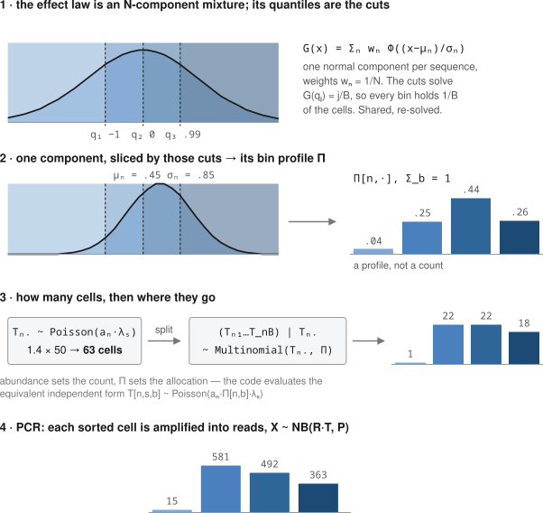
X[n,s,b] | T[n,s,b] ~ NB(R[s,b] · T[n,s,b], P[s,b])       reads from cells
T[n,s,b]            ~ Poisson(a_n · Pi[n,b] · lambda_s)   cells in bin b
Pi[n,b]             = Phi((q_b − mu_n)/sigma_n) − Phi((q_{b−1} − mu_n)/sigma_n)
Each sequence n carries a latent Gaussian effect law N(mu_n, sigma_n²) — its
expression distribution over cells — and an abundance a_n. The library's
marginal effect law is the N-component mixture of those per-sequence
normals, G(x) = Σ_n w_n Phi((x − mu_n)/sigma_n) with w_n = 1/N, and the B
sorting bins are its quantile cells: the cut points q_1 < … < q_{B−1} solve
G(q_j) = j/B. They are shared, and re-solved at every step, so every sequence
is tied to the marginal through them. This approach has 2 benefits: first one is that
it allows us to cut the number of params down to 2 instead of B-1, and the second one is that those params are further regularized, both by the normality assumption and the fact that they are all should form the global marginal distribution.
The activity that ships is the posterior mean of E[bin] = Σ_b b·Pi[n,b],
integrated over the posterior of (mu_n, sigma_n) with the abundance profiled
per grid point. The plug-in point estimate is a posterior mode, and for a
low-count sequence the mode sits at a simplex vertex — activity exactly 1 or
B, regardless of depth.
Install
pip install ebin
or
pip install -e /path/to/package # or place this directory on PYTHONPATH
jax (GPU-version strongly recommended: pip install jax[cuda]), numpy, scipy and pandas are required.
xarray + h5netcdf are needed only for the netCDF export and matplotlib
only for the diagnostics. Everything runs in float64 as some parts of the algorithm require high precision, namely the tridiagonal eigenvalue solver for orthogonal polynomials.
Input
One row per sequence, a 3-level column header (cell line, replicate, bin):
seq,       A549,A549,A549,A549,A549,...
           rep1,rep1,rep1,rep1,rep2,...
           bin1,bin2,bin3,bin4,bin1,...
ACGT...,   112, 340, 88,  15,  97,  ...
(in other words, the tabular should be readable with pd.read_csv(..., header=[0,1,2]))
Bins are ordered by the number in their name. Cell lines are fitted independently. Empty fields are read as zero counts, not as missing data — some exports write every zero as a blank, and treating those as missin
Install
pip install -e /path/to/package # or place this directory on PYTHONPATH
jax (GPU strongly recommended), numpy, scipy and pandas are required.
xarray + h5netcdf are needed only for the netCDF export and matplotlib
only for the diagnostics. Everything runs in float64.
Input
One row per sequence, a 3-level column header (cell line, replicate, bin):
seq,       A549,A549,A549,A549,A549,...
           rep1,rep1,rep1,rep1,rep2,...
           bin1,bin2,bin3,bin4,bin1,...
ACGT...,   112, 340, 88,  15,  97,  ...
Bins are ordered by the number in their name. Cell lines are fitted independently. Empty fields are read as zero counts, not as missing data — some exports write every zero as a blank, and treating those as missing deletes the informative zeros of the low-abundance sequences.
Use
python -m ebin counts.csv -o activity.csv
from ebin import activity_table

table, results = activity_table("counts.csv", out="activity.csv")
table[("A549", "activity")]        # posterior-mean E[bin] per sequence
The CSV has two header rows, (cell line, field), one row per sequence, and
carries everything the model estimates per sequence:
| field | meaning |
|---|---|
activity |
posterior-mean E[bin] — the normalized value intended for downstream use |
activity_sd |
its posterior SD — per-sequence confidence |
activity_map |
plug-in mode, kept for reference only |
mu, mu_sd |
posterior-mean effect location and its standard error |
sigma, sigma_sd |
posterior-mean effect scale and its standard error |
abundance |
fitted size factor a_n |
n_eff |
posterior grid support — large means the estimate is diffuse |
tot |
total observed reads |
All of it comes from the same posterior weights, so the columns are mutually
consistent: activity is Σ_b b·bin_prob. mu and sigma are in gauge units
(median cut 0, first cut −1), so they are comparable across sequences within a
cell line. A subset is selected with --fields activity,activity_sd,tot (or
fields=[...] in the API).
The B−1 cut points are a property of the cell line, not of a sequence, so
they are not columns: cuts_table(results) returns them as one row per cell
line, and the CLI writes them next to the activity table as
<out>_cuts.csv. The gauge fixes the first two at −1 and 0, so what varies
between lines is where the upper cuts land (A549 0.990, MDA-MB-231 0.964).
Sequences with no reads at all in a cell line keep an activity (they are fitted
as structural zeros and land near the neutral prior mean, ~2.5 for B = 4);
sequences with no observed cell at all are NaN.
Useful CLI options:
--groups A549,HepG2        cell lines to run, in output order
--abundance gamma          integrate a_n out instead of fitting it
--zero-truncation          drop all-zero rows instead of fitting them
--grid 61x25               readout grid (n_mu x n_log_sigma)
--save-fits fits.pkl       keep the fitted parameters
--warm-from fits.pkl       start from an earlier fit of the same data
--netcdf activity.nc       also write the full posterior (see below)
--plots DIR                also write the diagnostic plots
Per-bin distribution
The one field too wide for a flat table is bin_prob, the posterior-mean
probability of each bin — an (N, B) array per cell line. It is returned in
results, and --netcdf writes it alongside every scalar field:
from ebin import activity_table, write_netcdf

table, results = activity_table("counts.csv")
results["A549"]["bin_prob"]                    # (N, B), rows sum to 1
write_netcdf("activity.nc", results, table.index)
Readouts can be redone from saved fits without refitting, which is the cheap way to try a different grid or prior:
from ebin import readout_table
table, results = readout_table("counts.csv", "fits.pkl")
Diagnostics
Three plots, one panel per cell line, drawn from the table alone (--plots DIR
on the CLI writes all three):
from ebin import (plot_marginal_distribution, plot_activity_vs_raw,
                  plot_gc_vs_abundance)

plot_marginal_distribution(table, out="marginal.png")
plot_activity_vs_raw(table, "counts.csv", out="vs_raw.png")
plot_gc_vs_abundance(table, out="gc.png")
plot_marginal_distribution — the marginal effect law: the N-component
mixture G(x) = Σ_n w_n Phi((x − mu_n)/sigma_n), one normal per sequence,
drawn as the density it defines and sliced into the sorting bins, each in its
own colour. The x ticks are the cut points with their values. Weights are
uniform by default, as in the fit; weights= takes a per-sequence weight (the
fitted abundances, say) to see the marginal over cells rather than over
sequences. Every slice holds exactly 1/B of the mass by construction, so the
gauge (cuts at −1 and 0) and any unusual tightness or skew in a cell line's
effect law are visible here.
plot_activity_vs_raw — fitted activity against the depth-normalized raw
mass centre (each replicate×bin column divided by its own library size, then
Σ_b b·p_b), coloured by fitted abundance. Well-measured sequences sit on the
diagonal; the horizontal band at the centre is the low-abundance tail, where the
raw estimate is noise and the model shrinks toward neutral. A cell line whose
high-abundance sequences leave the diagonal is a real warning sign.
plot_gc_vs_abundance — GC content against the fitted size factor, with the
binned median trend. A strong trend means a_n is absorbing a
cloning/sequencing bias rather than biological abundance alone. GC is taken from
the table index when the index is the sequence; otherwise it is supplied through
sequences=.
raw_mass_center(counts) and gc_content(seqs) are exported separately for
cases where the raw numbers are more appropriate than a picture.
Configuration
Defaults are the shipped configuration; they are not arbitrary and are worth understanding before they are changed.
| option | default | why |
|---|---|---|
conditional |
False |
Zero inflation: all-zero rows are fitted with a structural-zero probability phi, so they enter the mixture that sets the cuts. Zero truncation (True) drops them, which sets the cuts on a zero-excluded distribution — measurably worse, both in-library and on transfer to an independent library. |
abundance |
True |
A free size factor a_n per sequence. Without one, every sequence has the same expected latent total, so real depth variation has nowhere to go but Pi — which tilts toward the bins with the largest channel scale, and Pi stops being a profile. |
abundance_prior |
None |
'gamma' integrates a_n out under Gamma(kappa, mean=1) instead: 2 parameters per sequence instead of 3, low-count sequences regularized, and the abundance uncertainty propagated into the effect. The activity profile is essentially unchanged (ρ ≈ 0.9996 against free a_n), so this is a parameter-economy. Costs ~2× runtime. |
mu_prior |
1.3 |
SD of the prior on the effect location. Bounding the effect spread alone still lets a single-bin low-count sequence run mu_n large and walk Pi to a vertex. The gauge pins Q50 = 0 and Q25 = −1, so the population SD is ≈ 1.5 and the between-sequence SD ≈ 1.1 — the gauge-consistent tau is ~1.3. A larger value (2–3) is inconsistent with the gauge and under-regularizes. |
sigma_prior |
(0.0, 0.5) |
Prior on log sigma_n. The per-sequence MLE is unbounded: a sequence whose reads land only in the outer bins wants a two-point mass, reachable only as sigma → ∞. Without this, sigma hits its bound in several cell lines; those are bad optima, so the prior often improves the data likelihood. (0, 1) fits marginally better on well-behaved lines but leaves stuck ones stuck. |
lambda_fix |
50.0 |
The latent Poisson level is not identified upward — it rides the R·lambda ridge, and only products like R(1−P)/P · Pi · lambda are identified. It is held fixed and R absorbs the scale. |
a_max |
15.0 |
Bound on a_n; also sizes the truncated latent-count grid, so raising it costs runtime and memory. |
| readout grid | 121 × 33 |
(mu, log sigma) grid for the posterior mean. Converged in the bulk: doubling to 181 × 49 moves the median activity by 2e-6 (a handful of extreme low-count sequences move by up to 0.04), while halving to 61 × 25 moves it by 5e-3. |
The readout re-uses the fit's own priors by default, so the posterior mean is
coherent with the fitted model. A flat effect location is obtained with
readout=dict(tau_within=None), and mu_center=<array> shrinks toward a
per-sequence target (for instance the same sequence's consensus across cell
lines).
Reproducing the shipped tables
The shipped activity_zi_full.csv (30k sequences × 20 cell lines) is the
default configuration:
python -m ebin data.csv -o activity.csv --save-fits fits.pkl
Cell lines come out in the order they appear in the count table, and every field
is written. The shipped table carried only activity, activity_sd, activity_map, tot in an explicit cell-line order, so
python -m ebin data.csv -o activity.csv \
    --fields activity,activity_sd,activity_map,tot --groups A549,HepG2,MCF7,...
reproduces that exact layout. The extra columns are additional output, not a change to the numbers.
Checked against the shipped table three ways:
- Readout. Given the shipped fitted parameters,
readout_tablereproducesactivity,activity_sd,activity_mapandtotto4e-16— exact up to CSV round-off. - Objective. The log-likelihood and its gradient agree bit for bit with the original implementation at the same parameter point, for zero inflation and zero truncation, free and Gamma abundance — including the gradient through the implicit cut-point solve.
- Full refit. Most cell lines land on the shipped optimum (
max|Δ|on activity ≤ 1e-6). A few of the hardest lines do not: the objective is multi-modal there, and the optimizer can settle in a neighbouring basin, which moves individual sequences by up to ~1e-1 (Pearson r ≥ 0.9998 against the shipped column). This is a property of the problem, not of the repackaging — the original code has the same instability on the same lines (re-fitting HCT116 with it lands 13 nats from its own shipped value), and both implementations reproduce those lines when fitted on their own.
The external-library (lib2) target used the same fit with a smaller readout
grid, selected with --grid 61x25.
The Gamma-abundance variant was warm-started from the shipped fits, which is what makes it affordable, and used a shorter finishing schedule:
from ebin import activity_table
activity_table("data.csv", out="activity_gamma.csv", warm_from="fits.pkl",
               abundance=False, abundance_prior="gamma", n_abund_nodes=30,
               max_outer=1, finish_maxiter=2000, finish_rounds=4)
The CLI runs the same variant on the default schedule:
--abundance gamma --nodes 30 --warm-from fits.pkl.
Runtime
One cell line of 30k sequences × 4 bins takes ~2–4 min on a GPU (fit + readout)
and roughly 20× longer on CPU; the Gamma-abundance variant costs ~2× the
free-a_n fit. Memory is dominated by the latent-count grid
(a_max · lambda_fix wide); the likelihood scans over abundance/rate components
so only one is live at a time. XLA_PYTHON_CLIENT_PREALLOCATE=false is set on
import so JAX does not claim 75% of VRAM.
Parameters
| symbol | shape | role | what it is | example (A549) |
|---|---|---|---|---|
X[n,s,b] |
N×S×B | observed | reads counted for sequence n in channel (s,b) | 1686 median total |
T[n,s,b] |
N×S×B | latent | cells of n that landed in bin b — never observed, summed out | ~63 cells |
mu_n, sigma_n |
N each | per sequence | the sequence's expression law over cells, in gauge units | σ median 1.46 |
a_n |
N | per sequence | size factor: how many cells n contributes at all. Geometric mean pinned to 1, capped at a_max |
1.42 median |
Pi[n,b] |
N×B | derived | bin profile, rows sum to 1. Not free — read off (mu_n, sigma_n) and the cuts |
— |
q_j |
B−1 | shared | cut points = quantiles of the mixture G at j/B. Gauge pins q_1 = −1, q_2 = 0 |
−1, 0, 0.99 |
lambda_s |
S | fixed | cell level of replicate s. Not identified — rides the R·lambda ridge, so held fixed while R absorbs the scale |
50 |
R[s,b] |
S×B | per channel | NB size per latent cell: R·T is the shape of the read distribution |
12.7 11.4 11.6 20.1 |
P[s,b] |
S×B | per channel | NB probability. Small P = a noisier channel at the same depth |
.33 .32 .31 .52 |
phi |
1 | shared | probability a sequence is a structural zero (dropout, never a cell) | 8e−7 |
kappa |
1 | optional | Gamma shape when a_n is integrated out instead of fitted; CV = 1/√κ |
0.9 (variant) |
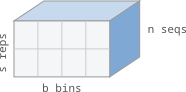
so X, T, R, P are 3D arrays:


Download files
Download the file for your platform. If you're not sure which to choose, learn more about installing packages.
Source Distributions
Built Distribution
Filter files by name, interpreter, ABI, and platform.
If you're not sure about the file name format, learn more about wheel file names.
Copy a direct link to the current filters
File details
Details for the file ebin-1.0.1-py3-none-any.whl.
File metadata
- Download URL: ebin-1.0.1-py3-none-any.whl
- Upload date:
- Size: 44.0 kB
- Tags: Python 3
- Uploaded using Trusted Publishing? No
- Uploaded via: twine/6.2.0 CPython/3.14.6
File hashes
| Algorithm | Hash digest | |
|---|---|---|
| SHA256 |
94c56d2ed7da15c33fa49864e4a22a30d5e1a26bf1d70ad741ba31c4bd8cd444
|
|
| MD5 |
631252808fcda8be5d74cbb32d0a7ae4
|
|
| BLAKE2b-256 |
bb438b10eac60eec1d00d885d28cb80e6eae3e43c69ad5ef367c7db3ff2f1065
|






