

Contributors: @VitorInserra · @Pranav1006 · @sainag7 · @Amit_Chalmeti · @ygadipalli
EEGProc
A lightweight Python library for EEG processing and deep learning, and model explanations. EEGProc is meant to be friendly to AI code writers and non-technical researchers, while still providing all the technical freedom and detail needed for EEG deep learning pipelines.
Built by researchers at the University of North Carolina (UNC) Chapel Hill and Columbia University, EEGProc has been used in research published at international conferences. It helps researchers and developers prepare EEG data, evaluate models, and explore their predictions with reusable, well-documented components.
We hope researchers will continue to contribute to this library, adding more model architectures, machine learning techniques, and visualization modules.
Install
pip install eegproc                   # preprocessing, features, conversion, plotting
pip install "eegproc[deep-learning]"  # adds models, cross-validation, counterfactuals
Requires Python 3.10 or newer. TensorFlow is optional and is installed with the
deep-learning extra.
Start with the DREAMER example
The commented example script walks through preprocessing, PSD feature extraction, a BiLSTM classifier, leave-one-subject-out cross-validation (LOSOCV), and a model-agnostic counterfactual for a held-out input.
Follow the example README for installation, dataset conversion, run commands, and an explanation of every step and output.
What EEGProc provides
- Preprocessing and features: filtering, detrending, spectral band powers, Hjorth parameters, and Shannon, wavelet, and IMF entropy.
- Dataset conversion: convert downloaded DREAMER, AMIGOS, EEGEmotions-27, and DEAP recordings into tidy CSV tables.
- Models and evaluation: reusable CNN/GNN components, RNN classifiers, classifier heads, losses, and subject-wise cross-validation.
- Model explanations: adapter-based counterfactual optimization for differentiable models, with plots and scalp topographies.
See the getting-started guide for focused API examples. The dataset guide covers supported layouts and download links; recordings are not bundled.
What can you model with EEG?
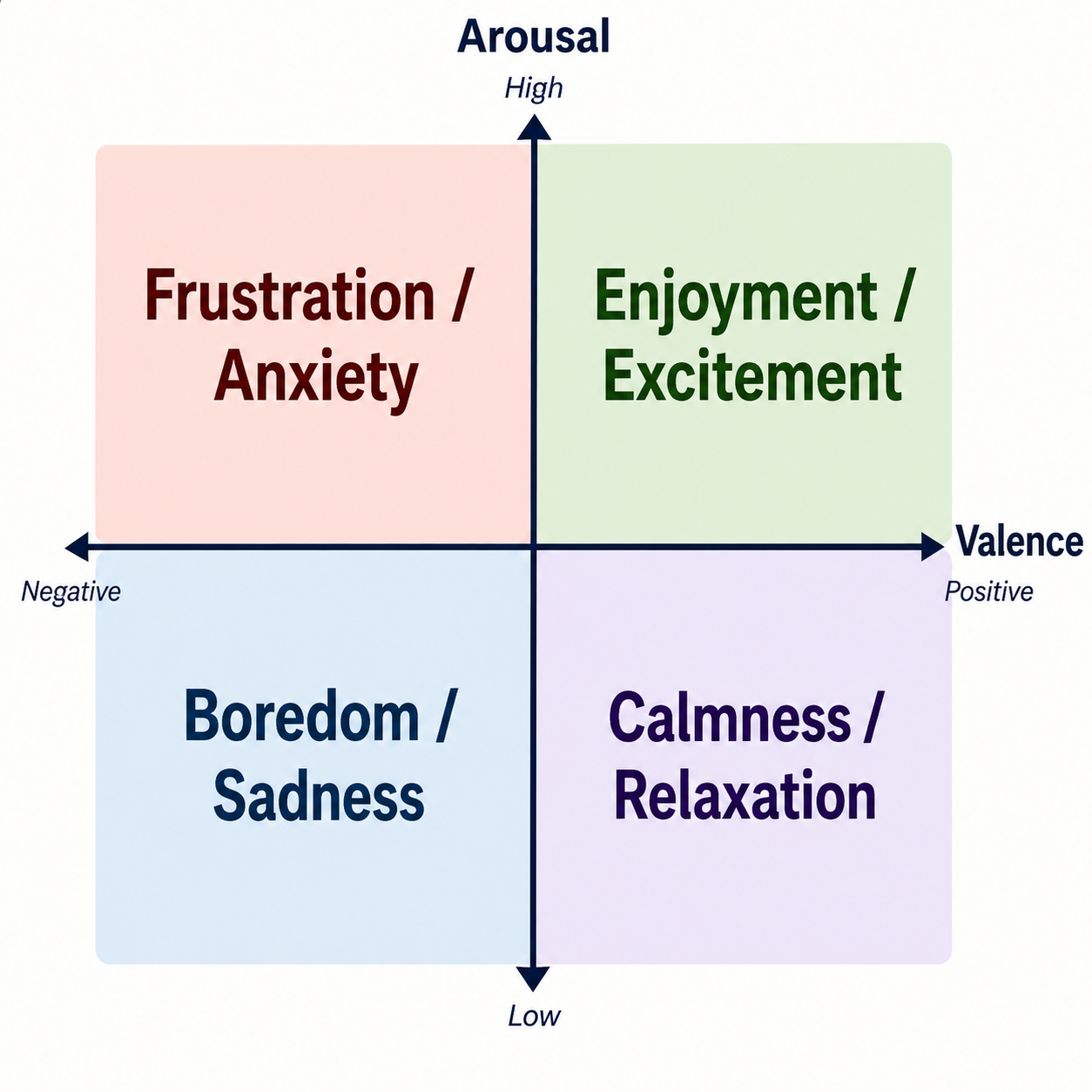
Developers and researchers can use EEGProc to build and evaluate models that estimate valence and arousal, attention, cognitive load, and engagement from EEG. Your labeled recordings, model, and evaluation protocol define the prediction task.
| Affective state | Cognitive state |
|---|---|
 |
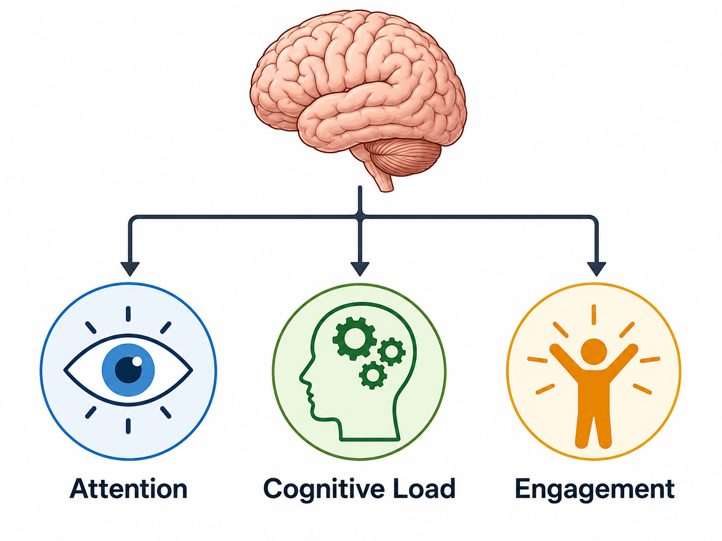 |
| Model affect along valence and arousal dimensions. | Estimate attention, cognitive load, and engagement. |
A typical EEG pipeline
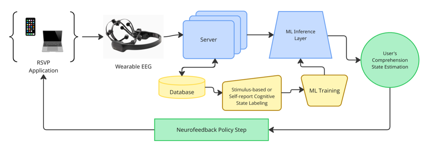
A typical workflow records EEG during a task, pairs recordings with labels such as self-reports or task measurements, and uses preprocessing and feature extraction to prepare model inputs. After training and subject-wise evaluation, a model produces state estimates that an application can use for feedback.
EEGProc supplies the preprocessing, feature extraction, model-building, evaluation, and explanation components in this workflow. Your project connects the recording device, data storage, server, and application feedback loop. The DREAMER example demonstrates the processing, training, evaluation, and explanation steps on a downloaded dataset.
Featurization
import pandas as pd
from eegproc import bandpass_filter, psd_bandpowers, shannons_entropy, FREQUENCY_BANDS

raw = pd.read_csv("my_eeg.csv")        # one column per electrode
fs = 128

clean = bandpass_filter(raw, fs, bands=FREQUENCY_BANDS)   # -> AF3_alpha, AF3_theta, ...
psd = psd_bandpowers(clean, fs, bands=FREQUENCY_BANDS)    # one row per window
entropy = shannons_entropy(psd)                           # -> AF3_entropy, F7_entropy
Featurizers compose in a pipeline: the band-energy functions consume a filtered signal, and the entropy functions consume the corresponding energy table.
| Function | Consumes | Emits |
|---|---|---|
bandpass_filter |
raw signal | {channel}_{band} |
psd_bandpowers |
filtered signal | {channel}_{band} |
shannons_entropy |
PSD table | {channel}_entropy |
hjorth_params |
filtered signal | {channel}_{band}_activity, _mobility, _complexity |
wavelet_band_energy |
raw signal | {channel}_{band}_wenergy |
wavelet_entropy |
wavelet energy | {channel}_wentropy |
imf_band_energy |
raw signal | {channel}_{band}_imfenergy |
imf_entropy |
IMF energy | {channel}_imfentropy |
Plot EEG features over time
Use plot_eeg_features for stacked channel traces, channel/band selection, and
image export. The examples below use psd and entropy from the featurization
section; the four-second windows and 50% overlap match those feature calculations.
from eegproc.plotting import plot_eeg_features

# Save theta and alpha band-power traces for two channels.
fig, axes = plot_eeg_features(
    psd, title="EEG band powers", channels=["AF3", "F7"],
    frequency_bands=["theta", "alpha"], seconds=4, overlap=0.5,
    save_path="bandpowers.png",
)

# Entropy has one value per channel; select channels without a band filter.
entropy_fig, entropy_axes = plot_eeg_features(
    entropy, title="EEG spectral entropy", channels=["AF3", "F7"],
    seconds=4, overlap=0.5, save_path="entropy.png",
)
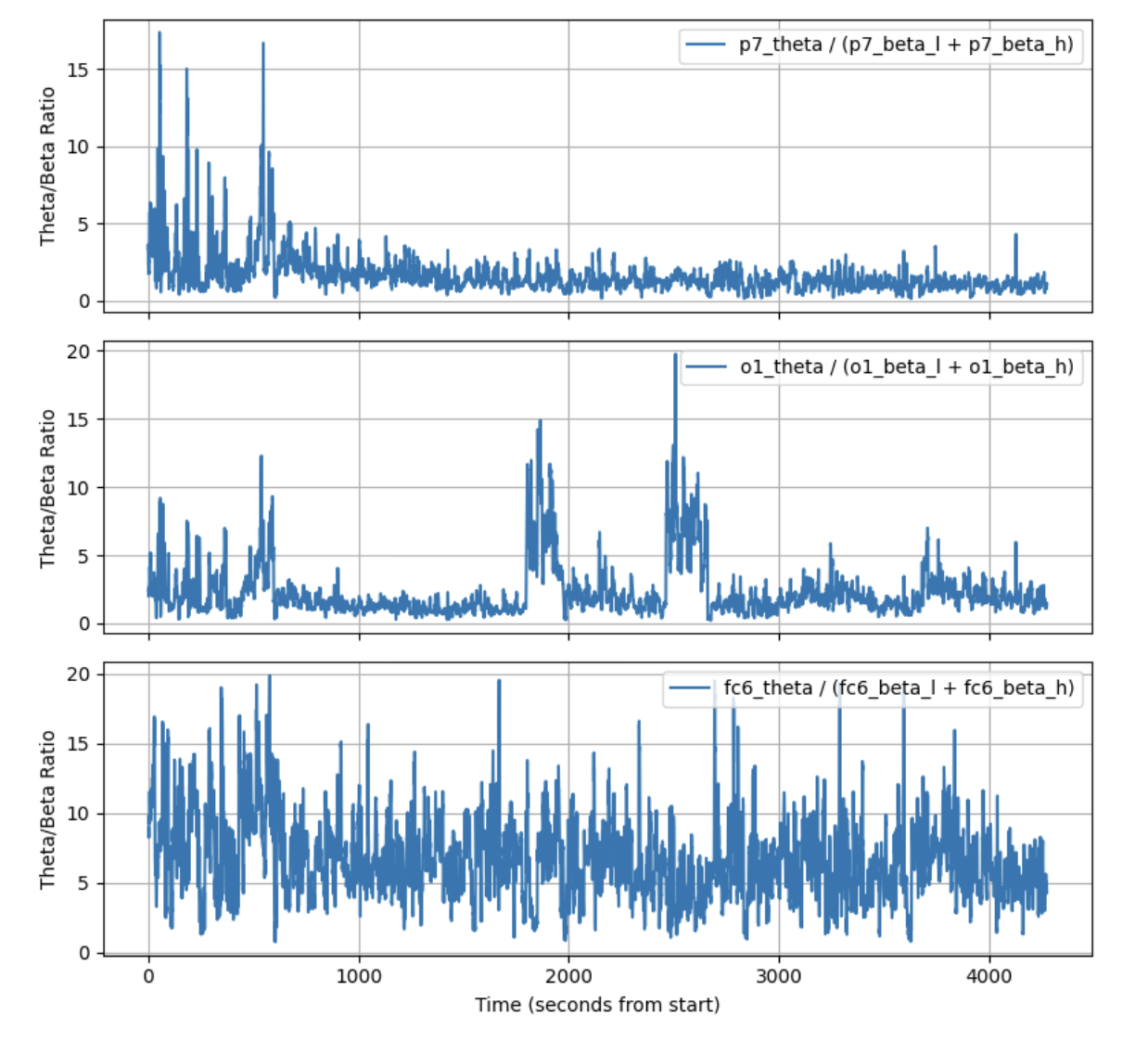
Illustrative EEG feature traces: theta-to-beta band-power ratios at P7, O1, and FC6. Derived ratios can also be passed to the plotting helper as a feature table.
Explain predictions with scalp topographies
EEGProc's model-agnostic module can visualize the differences between an input and its counterfactual across electrodes and frequency bands. Scalp topographies help show where those changes are concentrated.
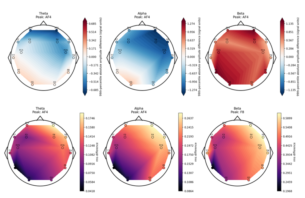
Example theta, alpha, and beta topographies: amplitude differences in the top row and root-mean-square (RMS) differences in the bottom row.
See the model-agnostic counterfactual guide for plotting commands and the channel positions, band metadata, and normalization information needed to interpret your own results.
Deep Learning
The DREAMER script builds a BiLSTM
and passes its builder to cross_validate_dataframe for leave-one-subject-out
cross-validation. Here is the same pattern for a prepared feature CSV containing
subject, trial, a binary label, and EEG features in time order:
import pandas as pd
from eegproc.deep_learning.supervised.rnn_architectures import BiLSTMClassifier
from eegproc.deep_learning.cross_validation import cross_validate_dataframe

features = pd.read_csv("features.csv")

def build_model(training_features):
    # Build a fresh BiLSTM using this fold's input dimensions.
    return BiLSTMClassifier(
        *training_features.shape[1:], n_classes=2, lstm_units=16, n_bilstm_layers=1,
    ).build()

results = cross_validate_dataframe(
    features, build_model, strategy="fixed_loso", fs=128,
    feature_columns=("AF3_alpha", "F7_alpha"),  # Choose your EEG features only.
    window_rows=4, normalize="subject_zscore",
    fixed_config={}, n_epochs=10, batch_size=32,
)
Each subject is held out once, with fixed training settings and windows kept
within trials. subject_zscore uses each subject's own unlabeled data, including
the held-out subject's data; omit it if that offline normalization assumption
does not fit your evaluation. Per-subject scores are in results["user_metrics"].
Follow the example README to run the complete DREAMER pipeline, including preprocessing, features, model saving, and counterfactuals.
Package layout
| Module | Purpose |
|---|---|
eegproc.preprocessing |
Filtering, detrending, and band decomposition |
eegproc.featurization |
Spectral, Hjorth, wavelet, and IMF features |
eegproc.data |
Dataset conversion, table schema, and trial-safe windowing |
eegproc.deep_learning |
Reusable models, cross-validation, and domain generalization |
eegproc.model_explainability |
Model-agnostic counterfactuals and topographies |
eegproc.plotting |
EEG feature plots |
Documentation and contributing
Browse the documentation, follow the contribution guide, or read the changelog. If you use EEGProc in your research, see CITATION.cff.
License
GPLv2. See LICENSE.
1 maintainer

Metadata
1 maintainer
Release files for eegproc 2.0.0
For a detailed explanation of source distributions (sdists) and built distributions (wheels), please see the package formats documentation.
Source distribution (sdist)
| File | Size | Uploaded | |
|---|---|---|---|
| eegproc-2.0.0.tar.gz | 200.8 kB | Details |
Built distribution (wheel)
| File | Interpreter | ABI | Platform | Reset |
|---|---|---|---|---|
| eegproc-2.0.0-py3-none-any.whl | Python 3 | none | any | Details |
Total release size: 433.0 kB
Release files / eegproc-2.0.0.tar.gz
| Download URL | eegproc-2.0.0.tar.gz |
|---|---|
| Size | 200.8 kB |
| Tags | Source |
|
SHA-256 checksum How to use checksums |
52972f494b7b923ce12e01f202e2cb6b4b2a5f61aa35a15a4e3d6a0620adb28f
|
|
BLAKE2b-256 checksum How to use checksums |
23a8da55d3db2146e01fb5d78c728493f5e5c15621b89dad358d9dbd84aa2538
|
| Upload date | |
|
Uploaded using Trusted Publishing? What is trusted publishing? |
Yes |
| Uploaded via |
twine/7.0.0 CPython/3.13.14
|
Provenance
Provenance describes where a file came from. On PyPI, provenance is shared via attestations, which provide a verifiable record of the build or publishing details. View details, limitations and caveats.


PyPI Publish Attestation
PyPI verified that this artifact, at this checksum, originated from the publisher listed below.
Signed by GitHub Actions, verified by PyPI on Oct 5, 2026.
Transparency logRelease files / eegproc-2.0.0-py3-none-any.whl
| Download URL | eegproc-2.0.0-py3-none-any.whl |
|---|---|
| Size | 232.2 kB |
| Tags | Python 3 |
|
SHA-256 checksum How to use checksums |
f77157c140407f87a43e3d5d0d198838b0c2e766ca2e786e9bc8c92ba182f763
|
|
BLAKE2b-256 checksum How to use checksums |
a5812131f19014923fd1bec9c50fc66f3a9c97146376279bb0aa1f1d00f5e0a2
|
| Upload date | |
|
Uploaded using Trusted Publishing? What is trusted publishing? |
Yes |
| Uploaded via |
twine/7.0.0 CPython/3.13.14
|
Provenance
Provenance describes where a file came from. On PyPI, provenance is shared via attestations, which provide a verifiable record of the build or publishing details. View details, limitations and caveats.
PyPI Publish Attestation
PyPI verified that this artifact, at this checksum, originated from the publisher listed below.
Signed by GitHub Actions, verified by PyPI on Oct 5, 2026.
Transparency log













