
An eXplainable AI package for tabular data.
Verified details
These details have been verified by PyPIProject links
GitHub Statistics
Maintainers

Project description
Effector







effector is an eXplainable AI package for tabular data. It:
- explains any black-box model with global and regional effects: what each feature does, and where the average hides something
- produces a report in one line:
effector.explain(X, model)fits, ranks the features, hunts for subregions, and writes a single self-contained HTML page - offers an interactive API when you want the controls: five engines (PDP, d-PDP, ALE, RHALE, SHAP-DP), one verb set
- is model agnostic: any callable
numpy → numpyworks, and adapters wrap scikit-learn, PyTorch, classifiers and DataFrame pipelines - is fast, for both global and regional methods: everything after the fit is free
📖 Documentation | 🚀 Quickstart | 🔧 API | 🏗 Examples
Installation
Effector requires Python 3.10+:
pip install effector
This installs a lightweight core (numpy, scipy, matplotlib, tqdm) that covers PDP, ALE, RHALE and their regional effects.
ShapDP needs the heavier shap/shapiq backends (which pull in numba, scikit-learn, pandas, ...). Install them only if you use that method:
pip install effector[shap]
Quickstart
(a) The inputs
A dataset as a numpy array, a model as a numpy → numpy callable, and, optionally, a schema so the explanation speaks your vocabulary:
import effector
from sklearn.ensemble import HistGradientBoostingRegressor

data = effector.datasets.BikeSharing()  # standardized numpy arrays
model = HistGradientBoostingRegressor(random_state=21).fit(data.x_train, data.y_train)
predict = effector.adapters.from_sklearn(model)  # a plain numpy -> numpy callable

schema = effector.Schema(
    feature_names=data.feature_names,
    feature_types=[
        "nominal", "nominal", "ordinal", "ordinal", "nominal", "nominal",
        "nominal", "ordinal", "continuous", "continuous", "continuous",
    ],
    category_names=[
        ["winter", "spring", "summer", "fall"],
        ["2011", "2012"],
        ["Jan", "Feb", "Mar", "Apr", "May", "Jun",
         "Jul", "Aug", "Sep", "Oct", "Nov", "Dec"],
        None,
        ["no", "yes"],
        ["Sun", "Mon", "Tue", "Wed", "Thu", "Fri", "Sat"],
        ["no", "yes"],
        ["clear", "mist", "light rain/snow", "heavy rain"],
        None, None, None,
    ],
    scale_x_list=[
        {"mean": data.x_train_mu[i], "std": data.x_train_std[i]}
        for i in range(data.x_train.shape[1])
    ],
    scale_y={"mean": data.y_train_mu, "std": data.y_train_std},
    target_name="bike-rentals",
)
📄 In depth: the input layer; pandas, sklearn, torch, classifiers, feature types, units.
(b) The one-liner
report = effector.explain(
    data.x_train, predict, y=data.y_train, schema=schema, nof_instances=5000
)
It fits once, ranks the features, hunts for subregions where the average is hiding something, keeps only the splits that pay for themselves, and opens with the one number worth having:
[effector] global effects   (GAM)  -> 72.3% of the model's variance
           regional effects (CALM) -> 92.0%
The result is a Report, a value you can export or print:
report.to_html("report.html")  # a single self-contained page; mail it, commit it
report.show()                  # the same story, as terminal tables
  ════════════════════════════════════════════════════════════════════════
  PDP report  ·  target: bike-rentals
  ════════════════════════════════════════════════════════════════════════

  DATA & MODEL
  ────────────────────────────────────────────────────────────────────────
    instances     5,000
    features      11  ·  5 nominal · 3 ordinal · 3 continuous
    model output  mean 188 · std 176 · range [-19.5, 948]
    model R²      0.960  (on this subsample)

  EXPLAINED VARIANCE
  ────────────────────────────────────────────────────────────────────────
    step         split on                 solo     ΔR²      R²       heter
    ──────────────────────────────────────────────────────────────────────
    GAM          (all features global)       —       —   72.3%           —
  + hr           temp, workingday, yr   +18.3%  +18.3%   90.6% 0.47 → 0.26
  + temp         hr, hum                 +2.4%   +1.4%   92.0% 0.22 → 0.19
    ──────────────────────────────────────────────────────────────────────
    FINAL                                                92.0%

  REJECTED SPLITS                                            min gain 1.0%
  ────────────────────────────────────────────────────────────────────────
    feature      split on                 solo     ΔR²    reason
    ──────────────────────────────────────────────────────────────────────
  ✗ yr           hr, workingday          +2.7%   -0.8%    redundant
  ✗ hum          hr, temp                +2.2%   +0.2%    below threshold
  ✗ weekday      hr, temp, yr            +0.4%   +0.2%    below threshold
  ✗ workingday   hr, yr                  +6.2%   -4.8%    redundant

    ✗ redundant: it would explain variance on its own (see solo),
      but the accepted splits already account for it.

  FEATURES                                ranked, in the selected snapshot
  ────────────────────────────────────────────────────────────────────────
    feature        importance                          heter      #regions
    ──────────────────────────────────────────────────────────────────────
    hr                 0.7273  ██████████████████     0.2608             4
    yr                 0.2271  ██████                 0.2088             1
    temp               0.2098  █████                  0.1874             4
    hum                0.0932  ██                     0.1221             1
    ──────────────────────────────────────────────────────────────────────
    the features above carry 82% of the total importance mass
(the accepted partition trees follow)
📄 In depth: the report; the explained variance ledger, the triage plane, the regional analysis, every knob of explain(...).
(c) The interactive API
The same engine, as a live handle you query as you go:
pdp = effector.PDP(data.x_train, predict, schema=schema, nof_instances=5000)

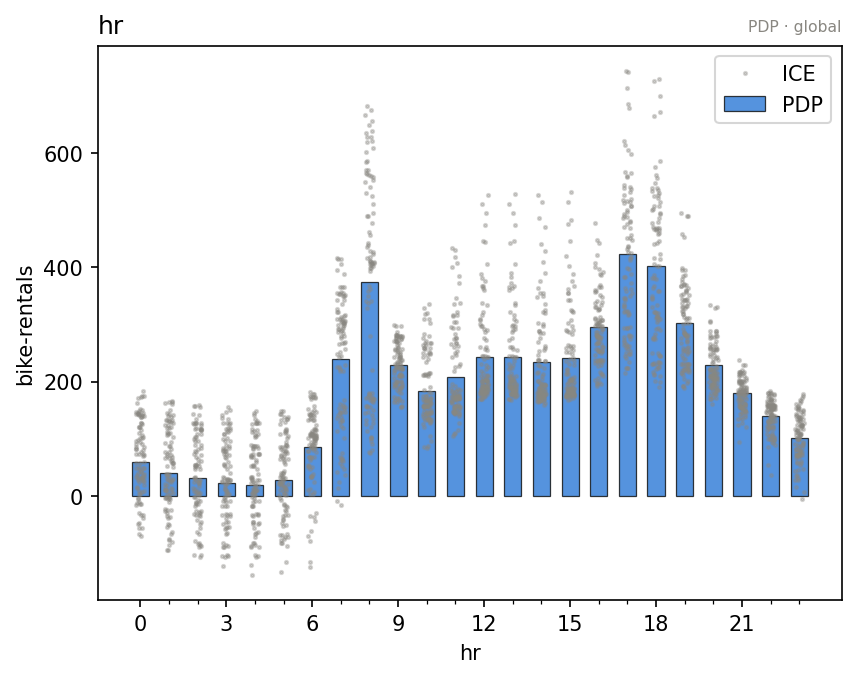
pdp.plot("hr")                        # the global effect, ICE curves behind it
pdp.heter_score("hr")                 # 0.47: the average hides a lot
partition = pdp.find_regions("hr")    # where is it hiding it?
partition.show()
Feature 3 - Full partition tree:
🌳 Full Tree Structure:
───────────────────────
hr 🔹 [id: 0 | heter: 0.47 | inst: 5000 | w: 1.00]
    workingday = no 🔹 [id: 1 | heter: 0.33 | inst: 1545 | w: 0.31]
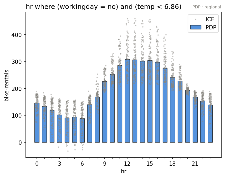
        temp < 6.86 🔹 [id: 2 | heter: 0.22 | inst: 778 | w: 0.16]
        temp ≥ 6.86 🔹 [id: 3 | heter: 0.26 | inst: 767 | w: 0.15]
    workingday = yes 🔹 [id: 4 | heter: 0.34 | inst: 3455 | w: 0.69]
        yr = 2011 🔹 [id: 5 | heter: 0.23 | inst: 1720 | w: 0.34]
        yr = 2012 🔹 [id: 6 | heter: 0.31 | inst: 1735 | w: 0.35]
--------------------------------------------------
Feature 3 - Statistics per tree level:
🌳 Tree Summary:
─────────────────
Level 0🔹heter: 0.47
    Level 1🔹heter: 0.34 | 🔻0.13 (28.12%)
        Level 2🔹heter: 0.26 | 🔻0.08 (22.91%)
The effect of hr depends on workingday (commute peaks vs a midday plateau), and within each branch on temp and yr. Plot the effect inside a region:
partition.plot(2) # hr, on non-working days, in the cold
 |
 |
Every verb answers one question:
| verb | question it answers |
|---|---|
.plot(f) |
what does feature f do? |
.eval(f, xs) |
…as numbers, on my grid |
.importance(f) |
how much does f move the output? |
.heter_score(f) |
is the average hiding something? |
.find_regions(f) |
where is it hiding it? |
.select_regions() |
which splits actually earn their keep? |
.fit(features, **cfg) |
(optional) tune the method first |
📄 In depth: the interactive API; construct and fit, customizing .fit(), plot, eval, scores, regions.
Documentation map
Start here:
- What are global and regional effects: the concepts
effector's API: the whole API in 3 minutes- (a) The input layer: numpy, models, adapters, the schema
- (b)
effector's report: the one-liner,.show(), and the HTML page - (c) The interactive API: the five engines, global and regional effects
Going deeper:
- The mental model: the thinking behind the API; one engine, values not state, two entrances
- Methods: the math reference: how each method defines the effect, its heterogeneity, and the two scalars
- The design contract: the rules the API is built on, one breath each
- Efficiency of global and regional methods: count the model calls
Supported Methods
Every method computes global effects, and regional effects via .find_regions(feature):
| Method | Class | Reference | ML model | Speed |
|---|---|---|---|---|
| PDP | PDP |
Friedman, 2001 | any | fast for a small dataset |
| d-PDP | DerPDP |
Goldstein et al., 2013 | differentiable | fast for a small dataset |
| ALE | ALE |
Apley & Zhu, 2020 | any | fast |
| RHALE | RHALE |
Gkolemis et al., 2023 | differentiable | very fast |
| SHAP-DP | ShapDP |
Lundberg & Lee, 2017 | any | fast for a small dataset and a light model |
Choosing a method
Three questions decide: is the dataset small (N < 10K) or large? Is the model light (< 0.1s per call) or heavy? Is it differentiable or not?
| your case | use |
|---|---|
| small + light | any: PDP, ALE, ShapDP; plus RHALE, DerPDP if differentiable |
| small + heavy | PDP, ALE; plus RHALE, DerPDP if differentiable |
| large + differentiable | RHALE |
| large + non-differentiable | ALE |
Citation
If you use effector, please cite it:
@misc{gkolemis2024effector,
  title={effector: A Python package for regional explanations},
  author={Vasilis Gkolemis et al.},
  year={2024},
  eprint={2404.02629},
  archivePrefix={arXiv},
  primaryClass={cs.LG}
}
Spotlight on effector
📚 Featured Publications
- Gkolemis, Vasilis, et al.
"Fast and Accurate Regional Effect Plots for Automated Tabular Data Analysis."
Proceedings of the VLDB Endowment | ISSN 2150-8097
🎤 Talks & Presentations
- LMU-IML Group Talk
Slides & Materials | LMU-IML Research - AIDAPT Plenary Meeting
Deep dive into effector - XAI World Conference 2024
Poster | Paper
🌍 Adoption & Collaborations
- AIDAPT Project
Leveragingeffectorfor explainable AI solutions.
🔍 Additional Resources
-
Medium Post
Effector: An eXplainability Library for Global and Regional Effects -
Courses & Lists:
IML Course @ LMU
Awesome ML Interpretability
Awesome XAI
Best of ML Python
📚 Related Publications
Papers that have inspired effector:
-
REPID: Regional Effects in Predictive Models
Herbinger et al., 2022 - Link -
Decomposing Global Feature Effects Based on Feature Interactions
Herbinger et al., 2023 - Link -
RHALE: Robust Heterogeneity-Aware Effects
Gkolemis Vasilis et al., 2023 - Link -
DALE: Decomposing Global Feature Effects
Gkolemis Vasilis et al., 2023 - Link -
Greedy Function Approximation: A Gradient Boosting Machine
Friedman, 2001 - Link -
Visualizing Predictor Effects in Black-Box Models
Apley, 2016 - Link -
SHAP: A Unified Approach to Model Interpretation
Lundberg & Lee, 2017 - Link -
Regionally Additive Models: Explainable-by-design models minimizing feature interactions
Gkolemis Vasilis et al., 2023 - Link
License
effector is released under the MIT License.
Powered by:
-
XMANAI


Project details
Verified details
These details have been verified by PyPIProject links
GitHub Statistics
Maintainers
Release history Release notifications | RSS feed


Download files
Download the file for your platform. If you're not sure which to choose, learn more about installing packages.
Source Distribution
Built Distribution
Filter files by name, interpreter, ABI, and platform.
If you're not sure about the file name format, learn more about wheel file names.
Copy a direct link to the current filters
File details
Details for the file effector-0.5.0.tar.gz.
File metadata
- Download URL: effector-0.5.0.tar.gz
- Upload date:
- Size: 160.6 kB
- Tags: Source
- Uploaded using Trusted Publishing? Yes
- Uploaded via: twine/6.1.0 CPython/3.13.12
File hashes
| Algorithm | Hash digest | |
|---|---|---|
| SHA256 |
2e30a339ce07641fea8f3b005441010e7e0786131058b2d527bb49df2f5ec24c
|
|
| MD5 |
5f448a5cf9ed3f0e8ffc983dd64331c1
|
|
| BLAKE2b-256 |
084276cf3721b5e0577ba5c8fcea0c39c83d7d6513715738433eb083d6d35dcb
|
Provenance
The following attestation bundles were made for effector-0.5.0.tar.gz:
Publisher:
publish_to_pypi.yml on givasile/effector
-
Statement:
-
Statement type:
https://in-toto.io/Statement/v1 -
Predicate type:
https://docs.pypi.org/attestations/publish/v1 -
Subject name:
effector-0.5.0.tar.gz -
Subject digest:
2e30a339ce07641fea8f3b005441010e7e0786131058b2d527bb49df2f5ec24c - Sigstore transparency entry: 2172750397
- Sigstore integration time:
-
Permalink:
givasile/effector@9bd1669e8f1bddc0e118b38ffbf684f453e0ca38 -
Branch / Tag:
refs/tags/v0.5.0 - Owner: https://github.com/givasile
-
Access:
public
-
Token Issuer:
https://token.actions.githubusercontent.com -
Runner Environment:
github-hosted -
Publication workflow:
publish_to_pypi.yml@9bd1669e8f1bddc0e118b38ffbf684f453e0ca38 -
Trigger Event:
push
-
Statement type:
File details
Details for the file effector-0.5.0-py3-none-any.whl.
File metadata
- Download URL: effector-0.5.0-py3-none-any.whl
- Upload date:
- Size: 170.6 kB
- Tags: Python 3
- Uploaded using Trusted Publishing? Yes
- Uploaded via: twine/6.1.0 CPython/3.13.12
File hashes
| Algorithm | Hash digest | |
|---|---|---|
| SHA256 |
1f6f3d458372a49a8db6965071ebee7007922e956c2d701467bf487c9b9e6f97
|
|
| MD5 |
2ec31ee8c65823d0d0bb38d74beed976
|
|
| BLAKE2b-256 |
650a351cc67c1614597f63cce1a9f80b72efa50b8bda7450498ea958bcc52214
|
Provenance
The following attestation bundles were made for effector-0.5.0-py3-none-any.whl:
Publisher:
publish_to_pypi.yml on givasile/effector
-
Statement:
-
Statement type:
https://in-toto.io/Statement/v1 -
Predicate type:
https://docs.pypi.org/attestations/publish/v1 -
Subject name:
effector-0.5.0-py3-none-any.whl -
Subject digest:
1f6f3d458372a49a8db6965071ebee7007922e956c2d701467bf487c9b9e6f97 - Sigstore transparency entry: 2172750440
- Sigstore integration time:
-
Permalink:
givasile/effector@9bd1669e8f1bddc0e118b38ffbf684f453e0ca38 -
Branch / Tag:
refs/tags/v0.5.0 - Owner: https://github.com/givasile
-
Access:
public
-
Token Issuer:
https://token.actions.githubusercontent.com -
Runner Environment:
github-hosted -
Publication workflow:
publish_to_pypi.yml@9bd1669e8f1bddc0e118b38ffbf684f453e0ca38 -
Trigger Event:
push
-
Statement type:






