





Automated exploratory data analysis and data-quality profiling for pandas DataFrames.
One function call (elessar.see(df), or elessar.see("sales.parquet")) or one command (elessar data.csv) gives
you the semantic type of every column, full descriptive statistics, the best-fitting distribution, associations
between all columns with significance tests, target and leakage analysis, feature selection, PCA and factor
analysis, outliers, time series, data-quality alerts and a preparation plan with the code to apply it, and
report-ready charts.
In Tolkien's legend, the Elessar is the green Elfstone through which whatever is seen is made whole again.
Every decision elessar takes (a column's type, whether a table is a time series, whether a date is a date of birth, whether PCA or a factor analysis is worth it, what to do with an outlier) is an explicit decision tree of named yes / no questions with stated thresholds, and the report shows the path each decision took. They are all drawn in How elessar decides.
Contents: What you get · Install · Quickstart · Any input, any size · API · How elessar decides · What it computes · Sample terminal output · Plots · Development
What you get
Pass a DataFrame, a file or almost anything tabular to see(), or a file to the elessar command, and get in
your terminal and in one HTML page:
- the semantic type of every column (not just the dtype): id, boolean in disguise, numbers stored as text, dates stored as text in any format, emails, URLs, phones, postal codes, IPs, JSON, free text, ordinal scales (low/medium/high, months, weekdays, 1-5 ratings), counts, integers that are really category codes (region 11, store 7, MCC 5411), mixed types… with the certainty of each decision
- dates of birth told apart from event dates, and turned into ages
- full descriptive statistics adapted to each type, with confidence intervals
- the best-fitting statistical distribution (MLE, ranked by AIC) and four normality tests
- associations of every kind with statistical significance: Pearson, Spearman, Kendall, Cramér's V, correlation ratio, mutual information, AUC, with p-values, Benjamini-Hochberg correction and confidence intervals
- target analysis: feature ranking, leakage detection, informative missingness
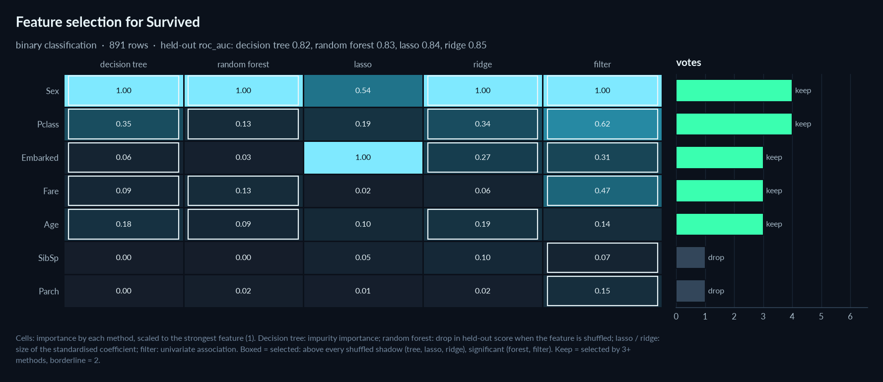
- feature selection by embedded methods (decision tree, random forest, lasso, ridge) and a filter, cross-validated, with a vote per feature
- multivariate statistics: whether PCA is worth it (Bartlett, KMO, parallel analysis), a factor analysis run step by step as it is taught (KMO and Bartlett, communalities, number of factors, varimax, Cronbach's alpha, scale scores), redundant groups of columns, rows that are outliers on several columns at once
- outliers found three ways (3 sigma, boxplot, modified z) and listed point by point, with whether to keep, remove or reassign them
- time series recognised on their own (single series, panel, event log): trend, stationarity, seasonality, decomposition, windows, validation folds on the real dates, augmentation recipes
- a preparation plan: every cleaning step (invalid values, wrong formats, misspellings, duplicates, consistency, missing data, outliers) and transformation (bucketing, decomposition, aggregation, combination, rescaling, normalisation, transformation, encoding, dimensionality reduction), each with its reason and its code
- data quality checks and actionable alerts (with the code to fix them): placeholders, duplicates, multicollinearity, values missing not at random, sorted rows…
- a set of plots that actually carry information, saved as PNG files, and one HTML page with everything
- any input, any size: CSV, Parquet, Excel, JSON, SQLite, SAS, Stata… or polars, pyarrow, dask, NumPy objects; files bigger than memory are typed progressively and streamed in parallel, with exact counts over every row
It is built for scripts and the terminal: plain-text output that fits your terminal width, files on disk, no display needed (except to click the target, if you ask for it).
Install
pip install elessar
The development version: pip install git+https://github.com/thibautdqb/elessar.
One install brings everything: pandas, NumPy, SciPy, Matplotlib, scikit-learn, dask, pyarrow (Parquet) and openpyxl / python-calamine (Excel). Requires Python ≥ 3.10.
Big files and dask. dask is installed with elessar and used automatically for files too big to load whole: it splits the file into blocks that are read and summarised on every core. Nothing to configure.
engine="pandas"/--engine pandasstreams in a single process instead.
Quickstart
import pandas as pd
import elessar

df = pd.read_csv("titanic.csv")

report = elessar.see(df, target="Survived")  # prints the report, writes the charts and the report page,
                                             # then opens the page in your browser
report.alerts                                # [{severity, column, message}, ...]
report.summary                               # one row per column, one column per metric
report.correlations["target"]                # features ranked, with tests, p-values, AUC, MI, leakage flag
report.multivariate["factor"]["steps"]       # the factor analysis, step by step
report.out_dir                               # elessar_report/df_target-Survived_2026-10-29/

elessar.see("data/*.parquet", target="ask")  # any file, glob or folder; pick the target in a window
elessar.see(polars_df), elessar.see(arrow_table), elessar.see(dask_df), elessar.see(numpy_array)
src = elessar.load("export.xlsx", sheet="2024")  # just the loader: src.df, src.full (exact figures), src.origin
Or straight from the shell (python -m elessar works too):
elessar titanic.csv --target Survived      # with a target
elessar titanic.csv --no-target            # without one
Run python examples/demo.py to see it on a deliberately messy synthetic dataset.
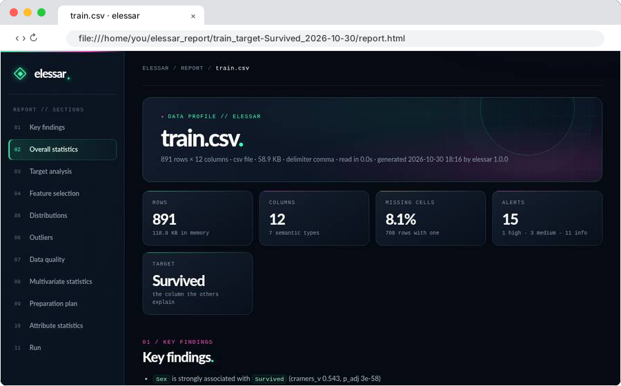
The report page
When the analysis finishes, elessar writes report.html next to the charts (and the same content as
report.md, which renders on GitHub, in VS Code, Obsidian…), and opens it in your browser. The page is a dark
"data observatory": a sidebar with every section numbered (the one you are reading lights up), key figures at the
top (rows, columns, missing cells, alerts, target), each chart in a card that opens full size on click, code
blocks with a copy button, and collapsible sections per column; it works offline, in one file with
--single-file, and on a phone. In order:
- key findings first: the features most associated with the target, then every high and medium alert
- overall statistics: the dataset overview, numeric and categorical columns at a glance, how each column was typed (its path down the decision tree and the certainty of the decision) and, for a sampled big table, the exact figures over every row
- target analysis: ranking with tests, AUC and mutual information, informative missingness, target charts
- feature selection: every method's importance per feature, the vote, the cross-validated score of each model, the lasso path
- time series (when the table is one): structure, trend, stationarity, seasonality, decomposition and autocorrelation charts, the per-entity table of a panel, the treatment and the validation folds
- distributions: for every numeric column the normality tests, the best fit with its parameters, Akaike weight, ΔAIC to the runner-up and the size of the misfit (KS D), next to histogram + fit + Q-Q charts
- outliers: the three methods per column, a chart of every flagged point, the most extreme points by row,
the rows that are outliers on several columns (
outliers.csvlists every flagged point) - data quality, including the checks on dates of birth
- multivariate statistics: PCA; the factor analysis as a checklist (each step, its question, its answer), the unrotated and rotated component matrices with communalities, Cronbach's alpha per factor with the alpha if each item is deleted, the new factors and their descriptives, and the code; groups of redundant columns; then the associations (heatmaps with significance, strongest pairs, linear dependencies, VIF)
- the preparation plan: cleaning then transformation steps, each with why and the code
- attribute statistics: one collapsible section per column with every statistic laid out in cards (center, spread, quantiles, shape, outliers, row order, labels, time, text), its normality tests, its top fits, its top values, its alerts with the fix, and its charts
- run details: source, how it was read, processes used, time per step, versions
StoneConfig(single_file_report=True) / --single-file also writes report_single.html with every chart
inlined: one file to send or attach.
Where it is written. Each run gets its own folder, elessar_report/<name>_<target>_<YYYY-MM-DD>/, named after
the file or the variable holding the DataFrame, and the target or its absence:
elessar trans.asc -t type → elessar_report/trans_target-type_2026-10-29/, elessar.see(sales) →
elessar_report/sales_no-target_2026-10-29/. Reports of different tables or targets never overwrite each other;
running the same analysis again on the same day refreshes that day's report. out_dir=... / -o FOLDER
writes to exactly that folder instead.
It opens automatically only when you run from a terminal, never in CI, tests or pipelines. Use
open_report="md" / --open md to open the Markdown file instead, or open_report=False / --open none to
never open it. report.to_markdown(path) and report.to_html(path) write it anywhere.
Choosing the target
The target is the column the others should explain (a label, a price, churn…). elessar never guesses it
silently. Give it with target="Survived" / --target Survived, or let a person pick: target="ask" opens a
small window listing every column, with the likely targets first (★, ranked by suggest_targets(df): names such
as target, label, churn, price, few classes, last column; identifiers and free text last). Double-click a
row or press Enter. Without a display it asks in the terminal. From the command line the picker opens by itself
when you run elessar data.csv interactively without --target (--no-target skips it).
Any input, any size
see() and elessar accept a pandas DataFrame / Series, a dict, a list of records, a NumPy array, a polars
DataFrame or LazyFrame, a pyarrow Table, a dask DataFrame, any object with the DataFrame interchange protocol,
and paths: a file, a URL, a glob pattern (logs/2024-*.csv) or a folder.
| Format | Extensions | Notes |
|---|---|---|
| delimited text | .csv .tsv .tab .txt .dat .psv |
delimiter (, ; tab |) and encoding (UTF-8, cp1252, Latin-1) sniffed |
| JSON | .json .jsonl .ndjson |
records, columns or lines |
| Parquet, Feather / Arrow, ORC | .parquet .pq .feather .arrow .orc |
|
| Excel, OpenDocument | .xlsx .xlsm .xls .xlsb .ods |
first sheet with data, or sheet= |
| SQLite | .sqlite .db |
biggest table, or table= |
| SAS, Stata, SPSS, HDF5, pickle, XML | .sas7bdat .xpt .dta .sav .h5 .pkl .xml |
Compressed files (.gz .bz2 .zip .xz .zst) are read directly; a file without a known extension is recognised by
its content.
Big tables
A table with more than max_rows rows (default 1,000,000), or larger than half of the free memory, is never
loaded whole. It goes through three steps:
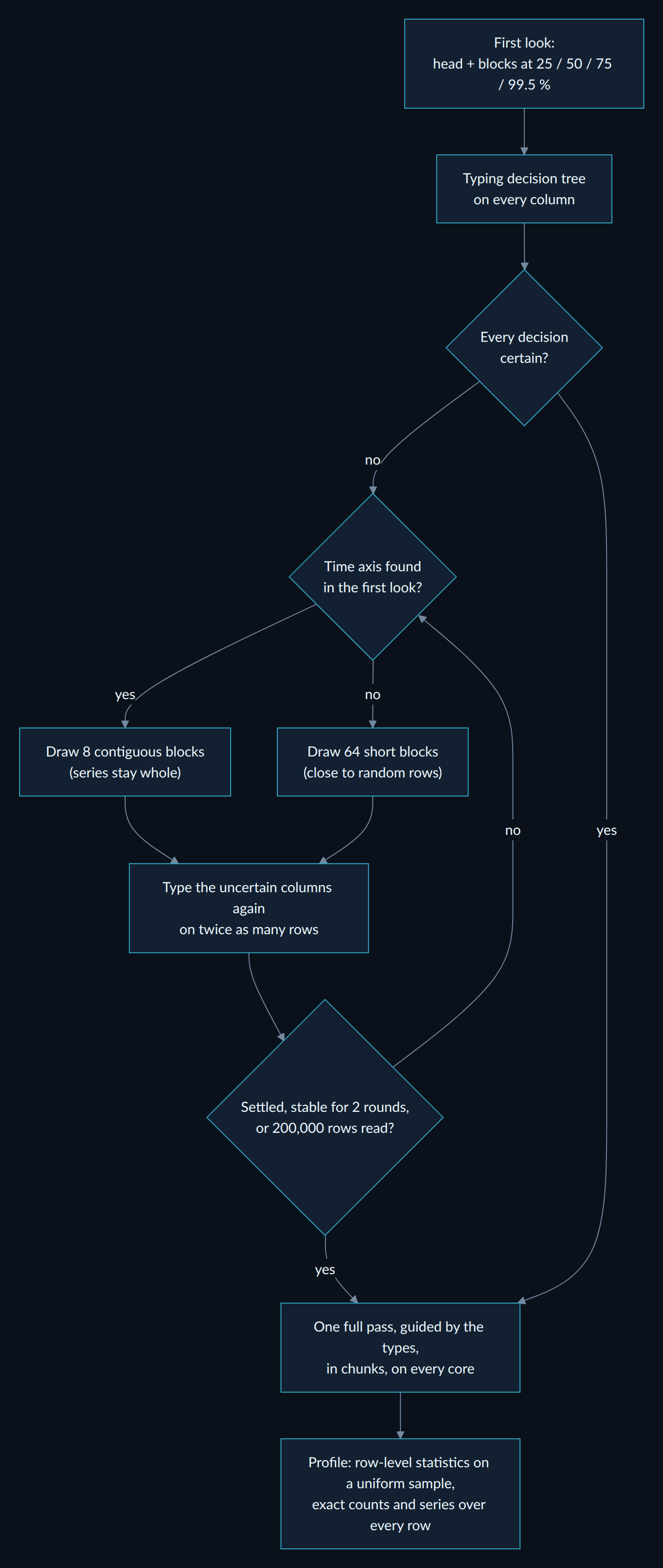
- Progressive typing. The types are decided before the full read, on as few rows as the evidence allows. Rows are reached directly (byte offsets in a text file, row groups in Parquet) and never read twice; the lines drawn from a text file are parsed together, so types come out as in a full read. When the first look finds a time axis, the extra rows are contiguous blocks, so series are never cut into scattered rows.
- One full pass guided by those types, in chunks, on every core; every chunk is reduced to a small summary:
- exact over every row: row count, missing values per column, min / max / mean / standard deviation (Chan's parallel algorithm) on the values the types say they are (numbers written as text parsed, dates read with their format), zeros, negatives, infinities, frequencies of low-cardinality columns, duplicate rows (64-bit row hashes), also ignoring the identifier columns;
- type checks over every row: values that do not fit their column's type, with their row numbers, and the uniqueness of every identifier, which no sample can prove. A decision that does not survive is corrected (an "identifier" that repeats becomes a grouping key) and reported;
- for a time-indexed table, the series aggregated per period over every row (counts, sums, means), and for a panel the active entities per period and whole entities drawn at random (Bernoulli sampling on a hash of the entity key), so temporal statistics never rest on a thinned sample;
- distinct counts: exact below 4,096 values, estimated above (k-minimum-values sketch, ~1.6 % error);
- a uniform random sample of
max_rowsrows without replacement (the rows with the smallest random keys), in the original order and indexed by original row number, on which the row-level profile runs.
- The profile, on the sample for row-level statistics and on the exact series for time.
Chunks are independent, so they are reduced on every core: CSV files are split into byte ranges by dask, Parquet files by row group, in-memory frames by slice. The report says the profile is sampled and shows the exact table.
Parallelism. The heavy steps (per-column statistics and distribution fits, every association test, the
advanced analyses, every chart) run as independent tasks on forked processes, one per core: the DataFrame is
inherited, never copied or pickled, and BLAS threads are limited to one per process. Results are identical to a
single-process run (a test checks it). Small tables stay in one process; StoneConfig(n_jobs=1) / -j 1
disables it, n_jobs=k caps it.
On macOS and Windows, where a process cannot be forked safely (Windows has no fork; on macOS it can crash the
numerical libraries), the chunks of a big file are read and summarised by fresh processes on every core instead
(they are self-contained: a byte range or a row group), even from a script without an
if __name__ == "__main__": guard; the other steps run in one process. Results are the same everywhere.
| Table (full run: every analysis, every chart, the report) | Time (14 cores) |
|---|---|
| Titanic, 891 rows × 12 | 4.5 s |
| 500,000 rows × 20, synthetic Parquet | 22 s (42 s in one process) |
| 8,000,000 rows × 8, 480 MB CSV | 25 s, 1.0 GB of RAM (read and exact pass over every row: 7 s) |
API
| Function | Returns | What it does |
|---|---|---|
see(data, target=None, config=None, plots=True, out_dir=None, verbose=True, open_report=None, name=None, **load_options) |
Vision |
Runs everything, prints the terminal report, writes the charts and the report page, opens it. data is anything load reads; target="ask" opens the picker. |
load(source, config=None, *, sheet, table, sep, encoding, columns, nrows, engine) |
Source |
Reads anything into .df (every row, or the sample of a big table), with .full (exact figures) and .origin. |
suggest_targets(df), pick_target(df) |
list, label |
Ranked target candidates; the window / terminal picker. |
parse_dates(series) |
Series |
Dates in any of the formats below, as datetimes. |
see_column(series, config=None) |
dict |
Everything about one column: type, stats, distribution, alerts. |
see_types(df) |
DataFrame |
Semantic type, pandas dtype, confidence, certainty, decision path, reason, and conversion suggestions (should-be-numeric / datetime / boolean / category, with the code). |
see_stats(df) |
DataFrame |
Descriptive statistics, one row per column. |
see_dist(df) |
DataFrame |
Normality verdict and top-3 fitted distributions for every numeric column. |
see_corr(df, target=None) |
dict[str, DataFrame] |
Every association matrix with its p-values, the ranked pairs, VIF, missingness tests, target analysis (keys below). |
see_quality(df) |
dict |
Every data-quality check, plus alerts. |
see_plot(df, out_dir, target=None) |
list[Path] |
Writes only the informative plots. |
Every function accepts a StoneConfig to change thresholds (alpha, missing %, correlation and VIF thresholds,
rare-category %, sample sizes, max_rows, probe_max_rows, candidate distributions, …) or to set a column's type
by hand: StoneConfig(column_types={"region": "categorical", "cylinders": "numeric_discrete"}) (numeric_continuous,
numeric_discrete, categorical, ordinal-candidate, id or text) replaces the decision tree for those columns.
Command line
elessar SOURCE [-t TARGET | --no-target] [-o FOLDER] [--type COL=TYPE ...] [--no-plots] [--single-file]
               [--sheet S] [--table T] [--sep SEP] [--encoding E] [--columns a,b] [--nrows N]
               [--max-rows N] [--engine {auto,dask,pandas}] [-j JOBS] [--sample N] [--alpha A]
               [--width W] [--json] [--markdown] [--csv] [-q] [--open {auto,html,md,none}]
SOURCE is a file, URL, glob pattern or folder in any format above. -t ask opens the target picker (it opens
anyway when you run interactively without -t). --type COL=TYPE (repeatable) sets a column's type by hand.
-V / --version prints the version. Without -o, the report goes to its dated folder in
elessar_report/ and the command prints where.
Vision
| Attribute / method | Content |
|---|---|
.overview |
shape, memory, dtype counts, duplicates, overall missing %; for a big table, how the types were decided (typing) |
.summary |
DataFrame, one row per column, one column per key metric |
.columns |
column → full detail dict (including path and certainty of its type) |
.correlations |
name → DataFrame |
.quality |
all quality checks |
.alerts |
list of {severity, column, message}, sorted high → medium → info |
.plots, .plot_index |
paths of the PNG files written; one {column, other, kind, path} record per chart |
.recap |
paths of report.html and report.md (and report_single.html) |
.out_dir |
the folder the run wrote to |
.full |
for a sampled big table: exact figures over every row, one row per column; else None |
.timings |
seconds per step: load, columns, associations, quality, advanced, charts, report |
.selection |
feature selection: table (importance per method, votes, decision), keep, borderline, drop, scores |
.multivariate |
pca; factor (verdict, reason, steps, loadings, unrotated, communality, removed, redundant, coherence, reliability, scores, descriptives, code); groups of redundant columns; multivariate outliers |
.outliers |
per numeric column the three methods and the action; points: every flagged point; summary |
.timeseries |
structure, per-series trend / stationarity / seasonality, treatment, folds; None if not a time series |
.preparation |
steps (kind, action, column, why, code), plus what the detectors found (misspellings, groups, bins...) |
.print(), .render(width) |
the terminal report |
.to_dict(), .to_json(path), .to_csv(path), .to_markdown(path), .to_html(path) |
exports (CSV = the summary table) |
How elessar decides
Each tree below is the code's own order of questions; the first yes decides. Thresholds are constants in the
code and fields of StoneConfig.
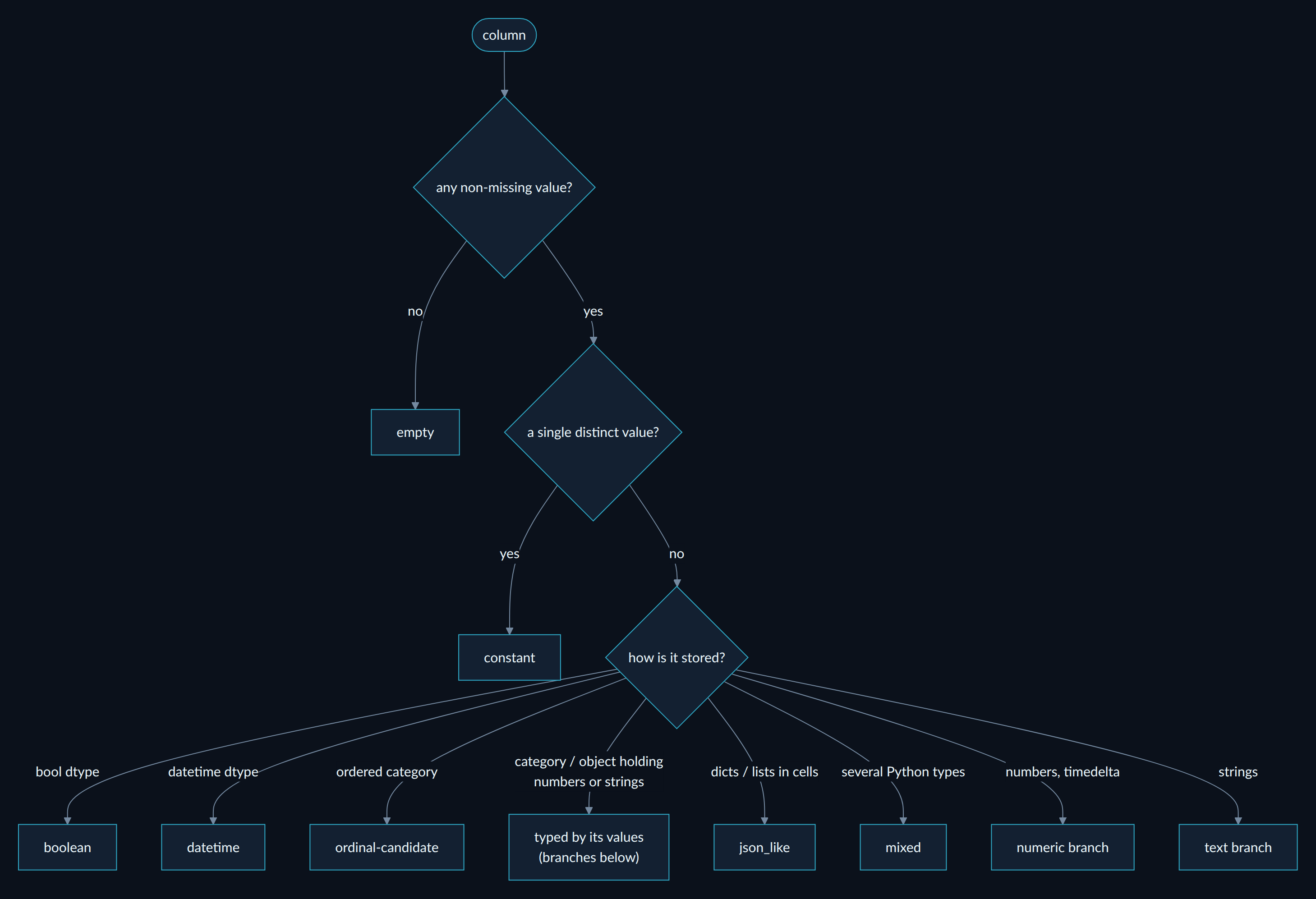
1. The type of a column
A column is first routed by how it is stored, then goes down the numeric or the text branch:
| Numeric branch: first yes wins | Type | Text branch: first yes wins | Type | |
|---|---|---|---|---|
| only 0 and 1? | boolean |
two boolean-like labels (yes/no, oui/non, y/n…)? | boolean |
|
| dates written as numbers (YYYYMMDD, Unix time…)? | datetime_string |
JSON objects or arrays? | json_like |
|
| an identifier by its name? | id (or a grouping key if it repeats) |
e-mail addresses? URLs? IP addresses? | email, url, ip_address |
|
| unique, consecutive or sorted integers? | id |
UUIDs? | id |
|
| integers that label categories (codes)? | categorical (probable) |
|||
| a small scale of consecutive integers? | ordinal-candidate or a count |
postal codes? | postal_code |
|
| integers? | numeric_discrete (or continuous with many levels) |
dates written as digits (YYMMDD…)? | datetime_string |
|
| a handful of distinct real values? | numeric_discrete |
numbers written as text ("1 234,5", "12%", "90 min")? |
numeric_string |
|
| real numbers | numeric_continuous |
dates, in any format? | datetime_string |
|
| phone numbers (and not dates)? | phone |
|||
lists of labels ("Comedies, Dramas")? |
multi_label |
|||
| unique short labels? | id |
|||
| free text? | text |
|||
| labels on a known ordered scale? | ordinal-candidate |
|||
| labels? | categorical |
|||
| otherwise | text (high cardinality) |
Every decision carries its certainty, shown in the report next to the path:
- certain: every value was seen, or, on a sample, each threshold test ("at least 90 % of the values are dates") holds at 95 % confidence (the Wilson interval of the observed share does not cross the threshold) and no label is likely unseen (Good-Turing estimate of the unseen probability mass, values seen once / values seen, below 1 %);
- probable: an identifier, empty or constant column decided on a sample: only every row can prove it, and the full pass does; or integers read as category codes: no number of rows can prove what an integer means;
- uncertain: a test whose interval crosses its threshold, a share of distinct values within 5 points of its threshold (not a proportion of independent draws, so no interval is claimed for it), few values, or an ambiguous day / month order. On a big file, uncertain columns are typed again on more rows (above).
Integers that are codes. A region 11, a store 7, a payment type 3, a merchant category 5411 or a
postal code 75011 are labels written with digits: their mean, standard deviation, correlation or "outliers"
mean nothing, and they belong with the categories (Cramér's V, chi-square, one-hot or target encoding). They are
recognised:
- by name: the first or last word of the column name is a category word (
region,store,dept,zip,mcc,naf,country,sex,gender,status,type,category,segment,cluster,group,mode,payment,channel,brand,origin… orcodewith another word:code_region,mcc_code), unless a word says the column counts or measures (n,count,total,price,amount,age,year,score,rating,level,defects,visits…:store_countstays a number); - by values alone: at most 50 distinct fixed-width integers of 3 digits or more, not years (1800-2100) and not rounded amounts (all multiples of 5), such as merchant or activity codes.
A graded scale starting at 0 in steps of 5 (0 / 5 / 10) is a score, never a code. These decisions are marked
probable, grouped in one alert, and can be reversed per column: StoneConfig(column_types={"store": "numeric_discrete"}) or elessar data.csv --type store=numeric_discrete. Checked on 1,007 columns of 65 real
tables: the only columns that change are gender coded 1 / 2 (three psychology datasets), and counts (SibSp,
cylinders, defect counts), years, prices, pulse rates and test scores stay numbers.
Dates, whatever the format: ISO 8601 with or without time and zone; day-first or month-first with any
separator (the order that parses every value wins, and a column where both work is reported as ambiguous); month
names in English, French, German, Spanish, Italian, Portuguese, Dutch and Czech; compact digits as text or numbers
(YYYYMMDD, YYMMDD, DDMMYYYY, YYYYMM, YYYYMMDDHHMM(SS), Czech / Slovak birth numbers with month + 50);
quarters (2020Q1) and ISO weeks (2020-W05); Unix timestamps in s / ms / µs / ns; Excel serial days when the
column name says it is a date. Two-digit years never land in the future. Zero dates (0000-00-00, 00/00/0000)
are placeholders for a missing date, never values. The suggested conversion uses the exact format found, and
elessar.parse_dates(series) does it in one call.
2. Is a date a date of birth?
A date of birth is a date, but not a time axis: it says who a row is about, not when something happened, and what models need is the age.
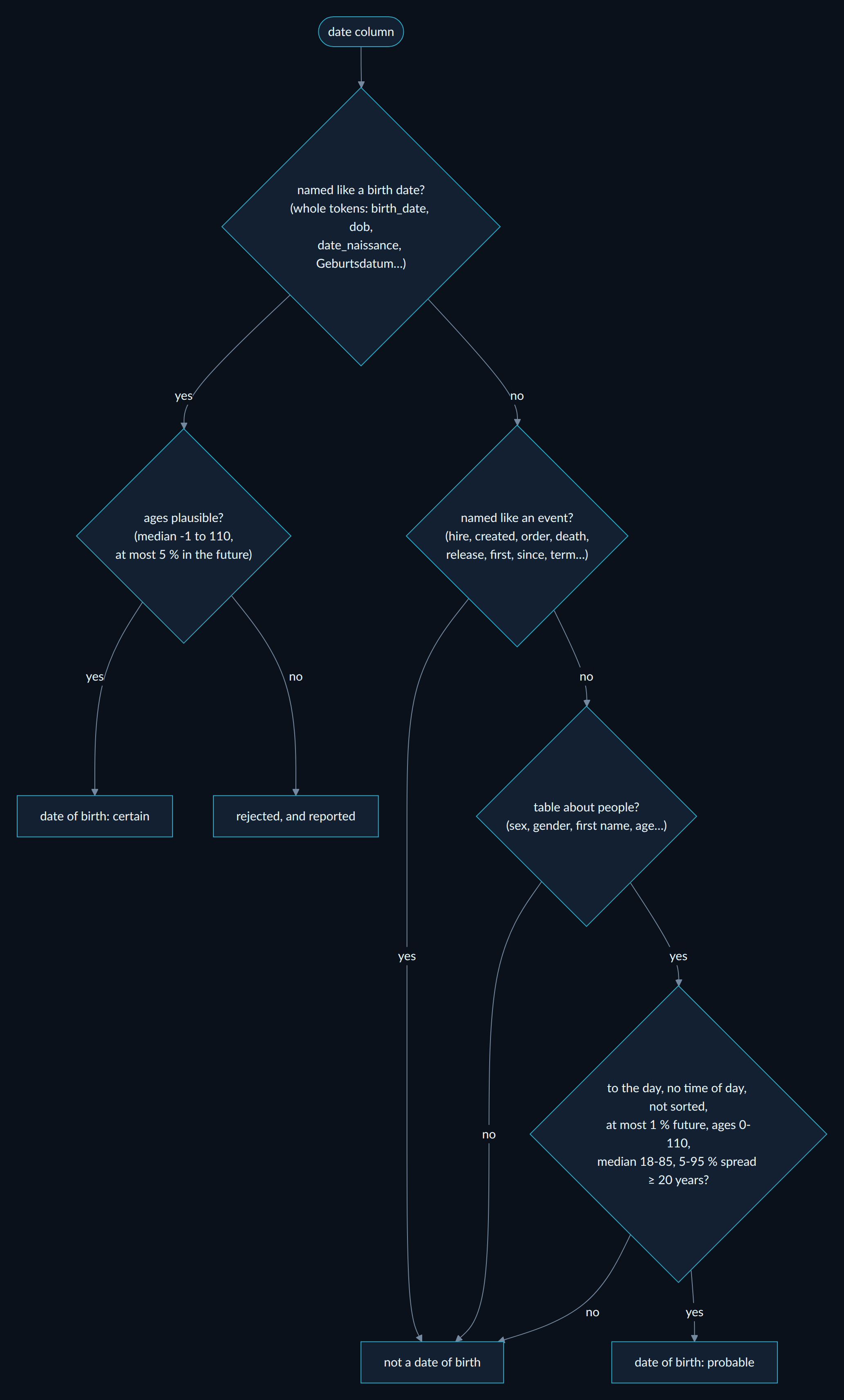
Each date of birth gets a derived age column, profiled and tested against the target like any other,
computed row by row at another event of the row when the table has one (age at admission, at the start of a term,
at an award year), else on the day of the analysis (which the report says). It is never used as a time axis, the
preparation plan models the age instead of the calendar parts, and it is checked: births after the reference,
ages above 120 at an event, an excess of 1 January or of first days of the month (one-sided binomial test against
the calendar share: day or month unknown), agreement with an age column (a constant gap dates the extract), the
share of minors, and a reminder that a date of birth is personal data and a strong quasi-identifier.
3. Is the table a time series, and of which kind?
Candidate time axes: a datetime column, dates as text, a datetime index, a year column, or year + month
columns (never a date of birth).
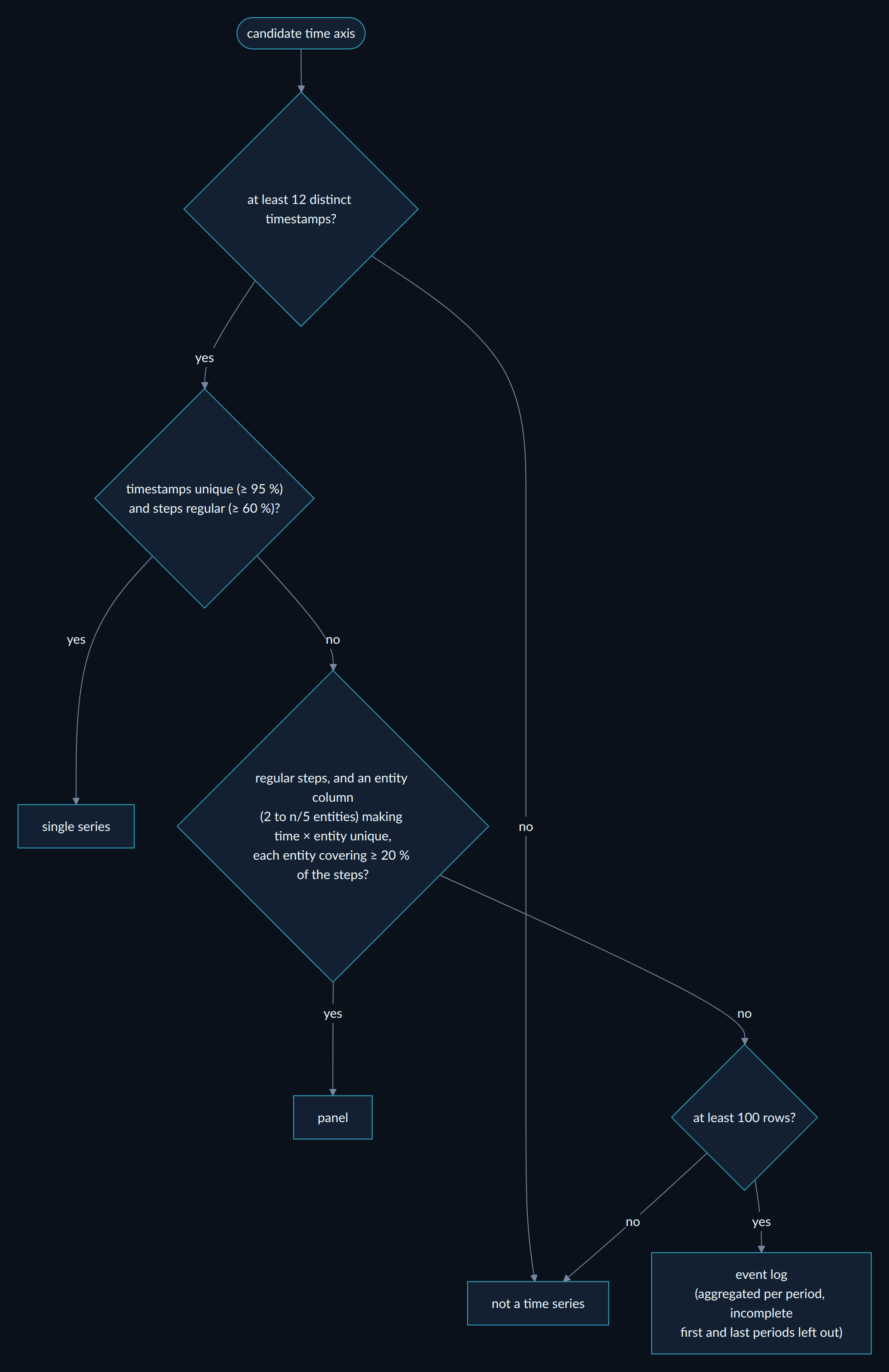
Then, per series:
- trend: Mann-Kendall test with the Hamed-Rao correction for autocorrelation (the uncorrected p-value of an autocorrelated series is far too small; the report shows both), Sen's slope;
- seasonality: a period natural to the frequency (7 / 30 / 365 days, 24 / 168 hours, 12 months, 4 quarters…) is screened on the autocorrelation of the detrended series (a peak, a dip before it, two full cycles) and kept when its seasonal strength from a classical decomposition reaches 0.25. The decision rests on this effect size: a significance test would itself be invalidated by the autocorrelation;
- stationarity: ADF (H0 unit root) and KPSS (H0 stationary), with and without a linear trend, read together on the seasonally adjusted series: stationary, trend-stationary (detrend, do not difference), unit root (difference) or inconclusive (break, changing variance, long memory);
- for a panel, the same tests on each entity's own series (whole entities drawn at random), with the share of entities with a significant trend after a Benjamini-Hochberg correction: a mean across entities would mix their dynamics with the change in which entities are present.
Treatment: ordering, gaps, aggregation, panel-safe lags, differencing or detrending as the tests say, Fourier terms, window and lag sizes, expanding-window validation folds computed on the real dates, augmentation for the training folds (jittering, scaling, window slicing, magnitude warping). The native resolution is kept up to 200,000 periods.
4. Is PCA worth it?
On the standardised numeric columns (target, identifiers, booleans and constants left out, missing values replaced by the median):
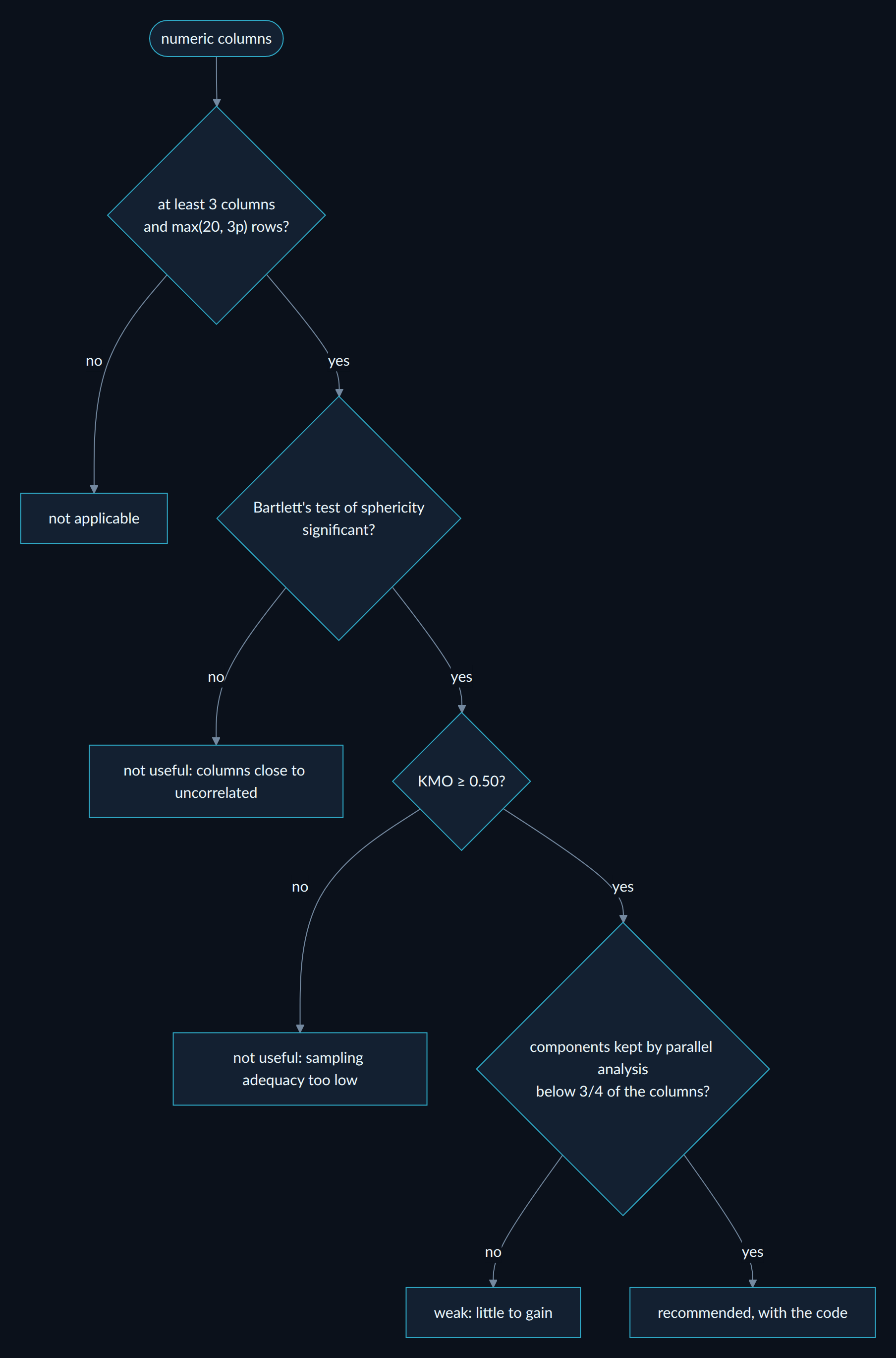
The report also gives Kaiser's rule and the components needed for 80 / 90 / 95 % of the variance.
5. Factor analysis, step by step
The factor analysis follows the method as it is taught and reported in SPSS-style studies. Each step is a line of the report's checklist, with its question, its answer and a yes / no / removed mark.
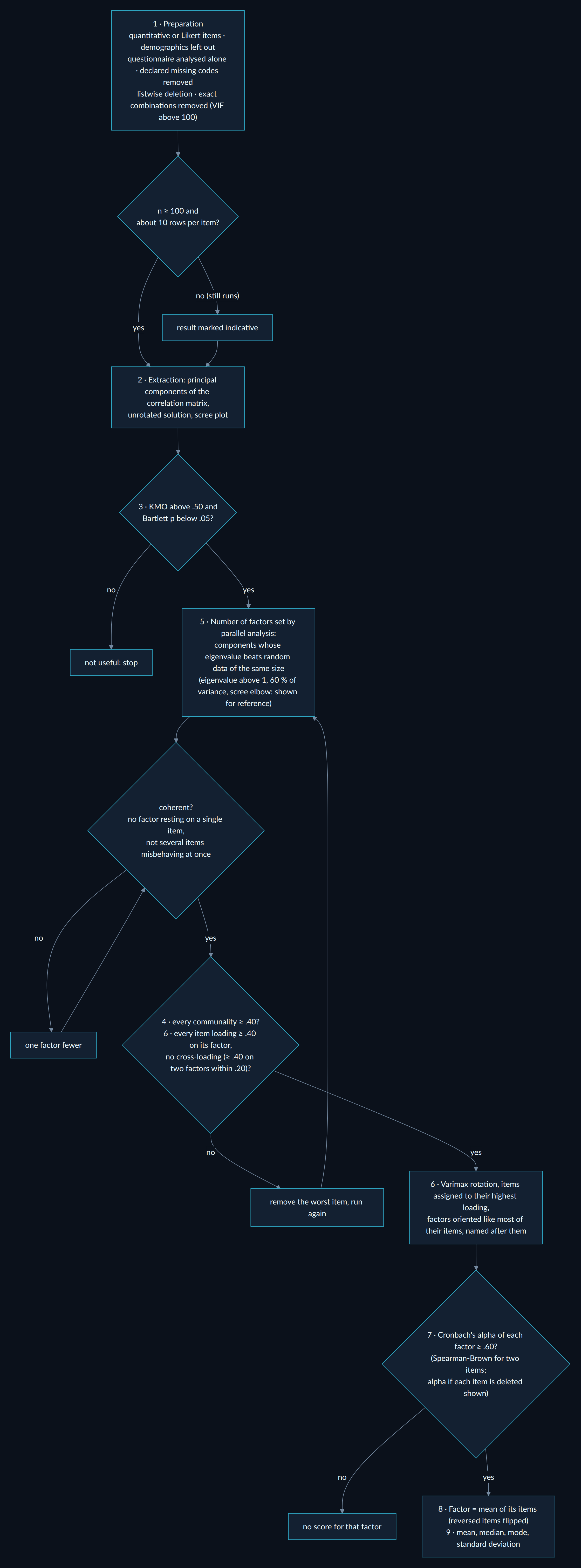
- Preparation. Items are quantitative or Likert variables: ordered labels such as disagree < neutral <
agree become their ranks; identifiers, booleans, dates, free labels and the target are left out, and so are
columns that describe the respondent rather than measure a construct (
age,sex,education,income,year…, recognised by their whole name:housing_median_agestays). When most of the variables are integer items on one response scale (a questionnaire answered 1 to 6), that questionnaire is analysed alone. Declared missing codes (-999…) become missing values, rows are deleted listwise, and an item that is an exact combination of others (a total, a mean of sub-items: VIF above 100) is removed, since it makes the correlation matrix singular. The determinant is reported against Field's 0.00001. Same scale for every item, or items standardised for the reliability and the scores. At least 100 complete rows and about 10 per item, otherwise the result is indicative. - Extraction: principal components of the correlation matrix, unrotated solution, scree plot, varimax rotation with Kaiser normalisation, loadings sorted by size.
- Pertinence: KMO above .50 and Bartlett's test below .05, on all the items and again on the items kept.
- Communalities (extraction): an item explained below .40 (Costello & Osborne, 2005) is removed and the analysis run again, one item at a time, the weakest first.
- Number of factors: eigenvalue above 1, cumulative variance of at least 60 % and the elbow of the scree plot (the eigenvalue farthest from the line joining the first and the last); the number two criteria agree on, else the scree plot. Then coherence: a factor resting on a single item is not a construct, and several items at fault at once usually mean too many factors rather than bad items, so one factor fewer is tried and kept when it leaves fewer items at fault.
- Rotated component matrix: each item goes to the factor of its highest loading; an item whose highest loading is below .40, or that loads at least .40 on a second factor within .20 of the first (cross-loading), is removed and the analysis run again. Each factor is oriented like most of its items, so the minority shows as reversed, and is named after its items.
- Cronbach's alpha per factor, reversed items flipped, with the alpha if each item is deleted: excellent ≥ .90, very good ≥ .80, good ≥ .70, acceptable ≥ .60, poor ≥ .50, else unacceptable. A deletion that would raise alpha by .05 or more is proposed, never applied: it must also make sense for the construct.
- New factors, only for the scales with an acceptable alpha: the mean of their items, with the code for the
mean of the answered items and for the version requiring every item (
MEAN.k). - Descriptives of the new factors: mean, median, mode, standard deviation.
The verdict is recommended when the factors pass every step and at least one reliable scale is created, indicative when the sample is small, not useful when KMO or Bartlett fail or no scale is reliable.
Checked on reference data sets whose structure is known: the 25 Big Five items of psych::bfi give the five
factors with the published keying (E1, E2, C4, C5, O2, O5 and A1 reversed) and alphas of .61 to .82, age and
education left out; Holzinger and Swineford's tests give the verbal, speed, spatial and memory factors; the mood
adjectives of psych::msq give the two arousal dimensions (energy and tension); one-factor scales
(Davis's drive for thinness, the breast-cancer biopsy scores, SAT / ACT, the beauty ratings of evals) give one
factor; aggregated trait scores (TIPI) and unrelated measures are found not useful.
6. What to do with an outlier
Per numeric column, three methods: 3 sigma (|x − mean| > 3 sd), the boxplot fences (Tukey, 1.5 IQR) and the modified z-score (Hampel, |0.6745 (x − median) / MAD| > 3.5). Every flagged point is listed with its row, value, z and robust z.
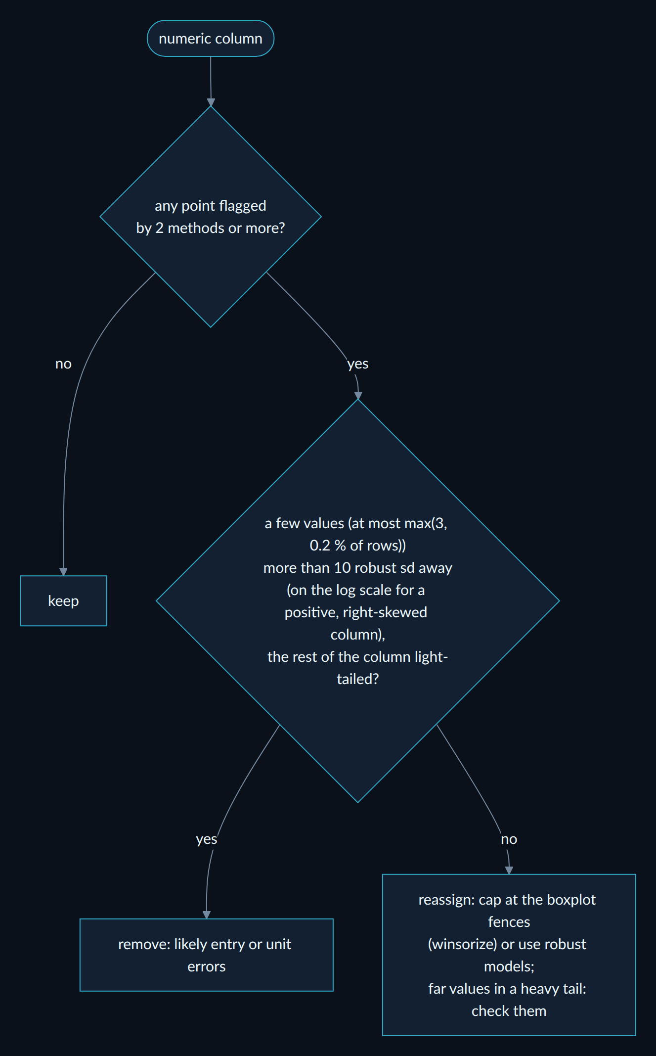
Multivariate outliers: robust Mahalanobis distance (minimum covariance determinant on Yeo-Johnson-normalised continuous columns, near-duplicates and linear combinations removed) beyond the chi-square 99.9 % quantile, confirmed by an isolation forest; flagged as indicative when more than 15 % of rows exceed it.
7. Which features to keep
With a target, the features (numeric, and categorical one-hot encoded but scored as one) go through five methods, after the features suspected of leakage are set aside:
| Method | Selected when |
|---|---|
| decision tree (depth chosen by cross-validation) | impurity importance at least half an equal share |
| random forest | permutation importance on held-out rows (all one-hot columns of a feature shuffled together) above twice its standard deviation |
| lasso (L1; L1 logistic regression for classes; penalty by cross-validation) | coefficient not zero |
| ridge (L2) | standardised coefficient at least 10 % of the largest |
| filter (univariate test) | significant after BH correction |
Selected by 3 methods or more = keep, 2 = borderline, else drop. Scores are R², ROC AUC (binary) or balanced accuracy, by 5-fold cross-validation, in time order for a time series.
What it computes
Semantic types: empty, constant, boolean (including 0/1, yes/no, true/false, y/n, oui/non), id
(unique or near-unique, consecutive ints, UUIDs), numeric_continuous, numeric_discrete (counts, few levels),
categorical (labels and high-cardinality codes), ordinal-candidate (low/medium/high, sizes, Likert, months,
weekdays, quarters, 1-5 integer scales, ordered categoricals), datetime, datetime_string, numeric_string
("1 234,5", "12%", "$3.2"), text, multi_label, email, url, phone, postal_code, ip_address,
json_like, mixed. Numbers written with units ("90 min", "60 kg") are parsed, and mixed units in one column
(min and Seasons, kg and lbs) are flagged.
Statistics
- all columns: count, missing, unique, memory, modes, top-N values
- numeric: caps / floors (censoring: values piled up at the max or min), zero inflation, mean (95 % CI), median (95 % CI from order statistics), std, var, sem, CV, min/max/range/sum, quantiles 1–99 %, IQR, MAD, 10 % trimmed mean, geometric and harmonic means, skewness, excess kurtosis, zeros, negatives, infinities, outliers (1.5×IQR, |z| > 3, modified z > 3.5), decimals, heaping (excess of round values, mixed-precision aware), monotonicity, lag-1 autocorrelation in row order with its p-value, bimodality coefficient, number of KDE modes
- categorical / boolean: cardinality, entropy, normalized entropy, Gini impurity, imbalance ratio, chi-square test of equal frequencies, share of True with its Wilson CI, rare categories, labels that differ only by case / spaces / accents, string lengths
- datetime: range, span, inferred frequency, largest gaps, duplicated timestamps, future dates, trend in rows per period (Kendall tau + p), distribution by year / month / weekday / hour (only when not trivial)
- text: length and word counts, empty / whitespace-only strings, share of digits / uppercase / punctuation, most common tokens
Distributions: Shapiro-Wilk, D'Agostino K², Jarque-Bera and Anderson-Darling with a majority verdict; MLE fits
of norm, lognorm, expon, gamma, weibull_min, beta, uniform, logistic, t, laplace, pareto, chi2, cauchy
(continuous) or poisson, nbinom, geom, binom (discrete), with support handling (shifted / rescaled fits), ranked
by AIC, with ΔAIC, Akaike weights, BIC and the KS statistic / p-value (KS p-values are optimistic when the
parameters are estimated from the same data: that is reported too). Integer data get a proper goodness of fit
(gap on the integer support, chi-square test) instead of KS, which ties inflate. A value holding 30 % or more of a
continuous column (rain: 57 % exact zeros) is reported as a point mass and the candidates are fitted to the rest;
fits that collapse onto repeated values are rejected. Each candidate has a timeout.
Associations and significance (see_corr keys)
| Key | Content |
|---|---|
pearson, spearman, kendall + *_p, n_numeric |
num-num matrices, their p-value matrices and pairwise-complete counts |
cramers_v + cramers_v_p + cramers_v_n |
bias-corrected Cramér's V with chi-square p-values |
eta + eta_p + eta_n |
correlation ratio (categorical rows × numeric columns) with Kruskal-Wallis p-values |
association, association_p |
one matrix over every column: Spearman, Cramér's V or eta depending on the pair |
pairs, top_pairs |
every pair tested (best method, n, test, p, BH-adjusted p, significant, Fisher 95 % CI), and those above corr_threshold |
vif |
variance inflation factor of each numeric feature (multicollinearity) |
linear_dependencies |
exact linear relations recovered as equations, e.g. Total = 1·HP + 1·Attack + 1·Defense + … |
missingness |
does a column go missing more for some values of another column? (Mann-Whitney / chi-square, BH-adjusted: evidence against MCAR) |
target |
each feature vs the target: association, test (Spearman / Kruskal-Wallis / Mann-Whitney / chi-square), p, BH-adjusted p, AUC (binary target), mutual information, leakage flag |
missing_target |
is the target different when a feature is missing? (informative missingness) |
Groups of columns with mean |Spearman| ≥ 0.7 are proposed for combination.
Preparation plan: cleaning: invalid values (placeholders, impossible values, infinities), wrong formats
(numbers or dates as text, mixed types, stray spaces, a file without a header row), misspellings (case, accents,
spaces, and 1-2 typos found with a BK-tree on the edit distance), duplicates (also ignoring identifier
columns), consistency (mixed units, values on two scales ~100× or 1000× apart), missing data (strategy by type and
by missingness mechanism), outliers to remove or reassign. Transformation: bucketing (numeric cut points from a
decision tree on the target; labels merged by a binary tree that only splits where the target differs
significantly, Bonferroni-corrected), decomposition (dates into calendar parts, dates of birth into ages, lists
into 0/1 columns, cells holding several data items such as "Paris, France" or "1920x1080" split), aggregation
(time series, panels), combination (redundant groups, exact linear relations, factor scores), rescaling,
normalisation, transformation of skewed columns (Box-Cox / log / Yeo-Johnson, with the skewness before and after),
encoding (by cardinality and type), dimensionality reduction (PCA or factor scores).
Quality: duplicate rows and columns, constant and quasi-constant columns, high missing, missing-value patterns
(columns that go missing together, rows with many missing, most frequent patterns), mixed types,
leading/trailing whitespace, placeholders used as missing ("", "NA", "null", "?", -999, 99999,
0000-00-00…), suspicious values (negative ages or prices, default dates like 1970-01-01), dates of birth (births
after the reference, impossible ages, 1 January excess), id-like columns, redundant columns, multicollinearity,
sorted rows, imbalanced target, dtype optimizations with the estimated memory saving.
Sampling inside the profile: on top of max_rows (above), expensive steps (correlations, Kendall, KDE,
pairwise tests, multivariate analyses) use at most sample_size rows (default 100 000); distribution fits and
normality tests use at most fit_sample_size values (default 20 000). Sampling is deterministic (random_state).
Robustness: elessar runs on any DataFrame, whatever the column names (empty, None, NaN, numbers, tuples /
MultiIndex, duplicates, slashes, newlines, emoji, pandas method names like count…) and whatever the content:
empty frames, a single row, all-NaN columns, inf and 1e±300 values, huge cardinality, lists / dicts / bytes in
cells, mixed types, sparse, nullable, categorical, period, interval, complex, Decimal, tz-aware datetimes,
timedeltas, duplicated or MultiIndex row index. The target can be given by its original label (tuple, number,
timestamp…). A randomized test suite generates hostile frames on every CI run. A failing step on one column is
recorded as an error entry and an alert; it never stops the report.
Real data: tested on 55 public datasets (Titanic, adult census, California housing, diamonds, Pokémon, Vega
movies, NYC taxis, penguins, wine quality, Netflix, Olympic athletes, Spotify, Nobel laureates, members of
Congress, a 62-column MultiIndex brain-network table…), on 17 reference datasets for the factor analysis, on the
Berka bank data (1 million transactions) and on an 8-million-row file. Things it finds there unprompted: Pokémon
Total = 1·HP + 1·Attack + 1·Defense + 1·Sp. Atk + 1·Sp. Def + 1·Speed; housing values capped at 500,001 and ages
at 52; adult capital gain top-coded at 99,999 and 92 % zeros; Titanic survival 30 % vs 67 % depending on whether
Cabin is missing; taxi tips always 0 when the payment type is missing; movie titles stored as numbers (300,
1776); Nobel laureates' and congressmen's birth dates, with their ages at the award or at the start of the term;
the five personality factors of the Big Five questionnaire; files sorted by price or year.
Sample terminal output
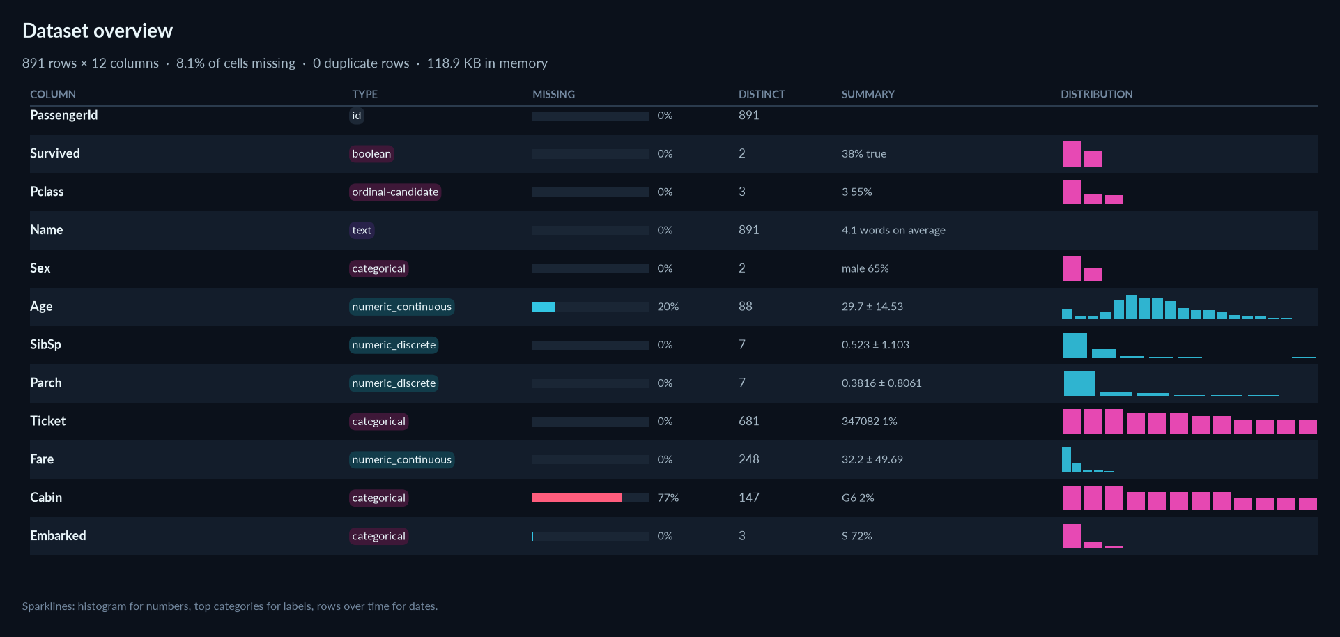
The Kaggle Titanic training set (elessar train.csv --target Survived), excerpt:
════════════════════════════════════════════════════════════════════════════════════════════════════════════════════
 elessar report  ·  891 rows x 12 columns
════════════════════════════════════════════════════════════════════════════════════════════════════════════════════

OVERVIEW
────────
  source          csv file · 58.9 KB · delimiter comma · read in 0.0s
  rows            891
  columns         12
  memory          118.9 KB  (suggested dtypes save ~53.7 KB)
  pandas dtypes   int64=5, str=5, float64=2
  semantic types  categorical=4, numeric_continuous=2, numeric_discrete=2, id=1, boolean=1, ordinal-candidate=1,
                  text=1
  duplicate rows  0 (0.0%)
  missing cells   8.1%  (708 rows with at least one)
  target          Survived

ALERTS (14: 1 high, 3 medium, 10 info)
──────────────────────────────────────
  HIGH    Cabin        77.1% missing -> drop, or impute and add a missing-indicator
  MEDIUM  Age          missingness is informative about 'Survived': Survived=1: 29% when missing vs 41% when present
                       (p_adj=0.0059) -> add a missing-indicator feature
  MEDIUM  Cabin        missingness is informative about 'Survived': Survived=1: 30% when missing vs 67% when present
                       (p_adj=6e-21) -> add a missing-indicator feature
  MEDIUM  Name         2 values with leading/trailing whitespace -> .str.strip()
  info    -            dtype optimizations save ~53.7 KB: PassengerId -> uint16, Survived -> uint8, Pclass -> uint8,
                       Sex -> category, Age -> float32, SibSp -> uint8, Parch -> uint8, Fare -> float32 (+1 more)
                       (see quality['dtype_optimizations'] for code)
  info    -            missing values are not random in 2 columns: Cabin (on Pclass), Age (on Embarked) -> see
                       correlations['missingness']; impute conditionally
  info    -            PCA recommended: 2 components (parallel analysis) keep 66% of the variance of 5 columns (KMO
                       0.54 miserable, Bartlett p 2e-153)
  info    -            104 rows are outliers on several columns at once (robust Mahalanobis + isolation forest) ->
                       inspect them (see Outliers)
  info    -            3 columns are heavily skewed (|skewness| > 2): SibSp, Parch, Fare -> details per column
  info    Cabin        high cardinality (147 categories) -> group rare levels or use target/frequency encoding
  info    Fare         13.0% outliers by the 1.5xIQR rule (outside [-26.72, 65.63])
  info    PassengerId  identifier-like column -> exclude from modelling and statistics
  info    SibSp        5.2% outliers by the 1.5xIQR rule (outside [-1.5, 2.5])
  info    Ticket       high cardinality (681 categories) -> group rare levels or use target/frequency encoding

COLUMN SUMMARY
──────────────
  column       type                missing  unique            mean/top  std/top%   min    max   skew
  ───────────  ──────────────────  ───────  ──────  ──────────────────  ────────  ────  ─────  ─────
  PassengerId  id                     0.0%     891                   1      0.1%
  Survived     boolean                0.0%       2                   0     61.6%
  Pclass       ordinal-candidate      0.0%       3               2.309    0.8361     1      3  -0.63
  Name         text                   0.0%     891  Braund, Mr. Owen …      0.1%
  Sex          categorical            0.0%       2                male     64.8%
  Age          numeric_continuous    19.9%      88                29.7     14.53  0.42     80   0.39
  SibSp        numeric_discrete       0.0%       7               0.523     1.103     0      8   3.70
  Parch        numeric_discrete       0.0%       7              0.3816    0.8061     0      6   2.75
  Ticket       categorical            0.0%     681              347082      0.8%
  Fare         numeric_continuous     0.0%     248                32.2     49.69     0  512.3   4.79
  Cabin        categorical           77.1%     147                  G6      2.0%
  Embarked     categorical            0.2%       3                   S     72.4%
...

COLUMN DETAILS
──────────────
...
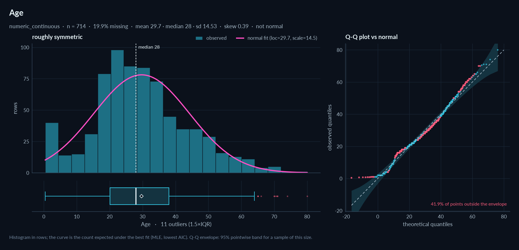
▸ Age  ·  numeric_continuous  ·  float64  ·  float64 dtype: 88 distinct real values
    missing 177 (19.9%) · unique 88 (12.3%) · memory 7.0 KB · mode 24.0 ×30
    mean 29.7 ± 14.53 · 95% CI [28.63, 30.77] · median 28 [27, 29] · trimmed 29.27 · IQR 17.88 · MAD 9 · CV 0.4891
    geo mean 24.43
    min 0.42 · p1 1 · p5 4 · p25 20.12 · p75 38 · p95 56 · p99 65.87 · max 80 · sum 21,205.2
    skew 0.389 · kurtosis 0.178 · outliers IQR 1.5% · |z|>3 0.3% · mod-z 0.1% · zeros 0 · negatives 0 · decimals 1
    heaping ×1.0 · KDE modes 1 · bimodality coef 0.36 · lag-1 autocorr 0.05 (p 0.19)
    normality: not normal · Shapiro p 7e-08 · D'Agostino p 1e-04 · Jarque-Bera p 8e-05 · Anderson p 0.01
    shape: roughly symmetric, best fit normal(loc=29.7, scale=14.5)
    #1 norm(loc=29.7, scale=14.5) AIC 5,850.5 KS p 0.005
    #2 t(df=22.9, loc=29.5, scale=13.9) AIC 5,851.3 KS p 0.016
    #3 logistic(loc=29.1, scale=8.15) AIC 5,851.4 KS p 0.046
...

CORRELATIONS
────────────
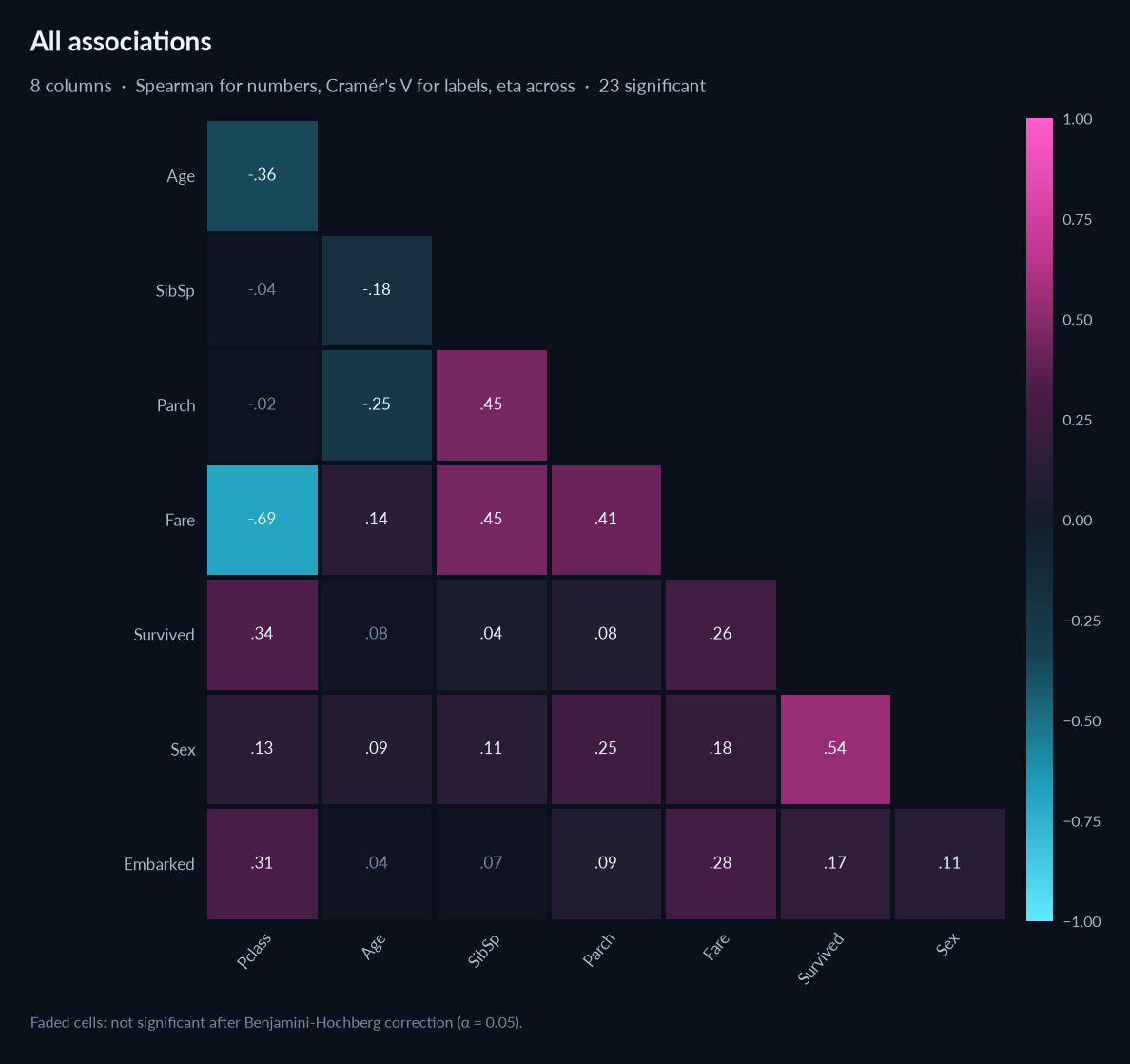
  28 pairs tested, 24 significant after Benjamini-Hochberg correction (alpha 0.05); strongest shown below
  column A  column B  method      value  95% CI              n   p_adj  sig
  ────────  ────────  ─────────  ──────  ────────────────  ───  ──────  ───
  Pclass    Fare      spearman   -0.688  [-0.725, -0.648]  891  2e-124  *
  Survived  Sex       cramers_v  +0.543                    891   5e-58  *

  multicollinearity (VIF): Pclass 1.7, Fare 1.6, Age 1.3, SibSp 1.3, Parch 1.2

  missingness that depends on other columns (evidence against MCAR):
    Cabin <- Pclass: median Pclass = 3 when missing vs 1 · p_adj 3e-91
    Age <- Embarked: 64% missing when Embarked=Q vs 14% when Embarked=S · p_adj 2e-23

TARGET ANALYSIS
───────────────
  target: Survived  (boolean)
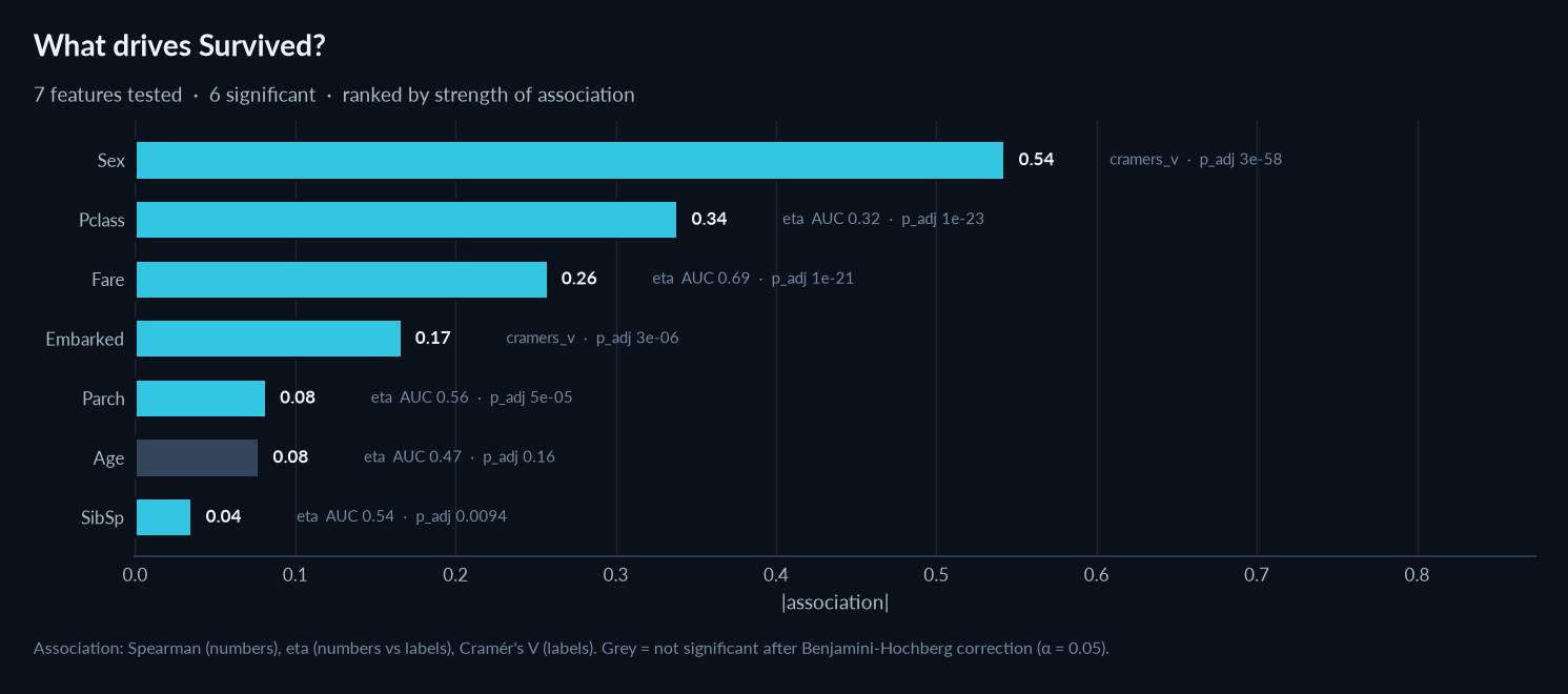
  feature   type                method     association  test            n   p_adj  sig    AUC     MI  flag
  ────────  ──────────────────  ─────────  ───────────  ────────────  ───  ──────  ───  ─────  ─────  ────
  Sex       categorical         cramers_v       +0.543  chi-square    891   3e-58  *           0.218
  Pclass    ordinal-candidate   eta             +0.338  mann-whitney  891   1e-23  *    0.319  0.092
  Fare      numeric_continuous  eta             +0.257  mann-whitney  891   1e-21  *    0.692  0.100
  Embarked  categorical         cramers_v       +0.166  chi-square    889   3e-06  *           0.021
  Parch     numeric_discrete    eta             +0.082  mann-whitney  891   5e-05  *    0.561  0.024
  Age       numeric_continuous  eta             +0.077  mann-whitney  714    0.16       0.469  0.023
  SibSp     numeric_discrete    eta             +0.035  mann-whitney  891  0.0094  *    0.543  0.019
  6/7 features significantly associated (BH-adjusted p < 0.05)

  is the target different when a feature is missing?
    yes  Cabin (77.1% missing): Survived=1: 30% when missing vs 67% when present · p_adj 6e-21
    yes  Age (19.9% missing): Survived=1: 29% when missing vs 41% when present · p_adj 0.0059

FEATURE SELECTION
─────────────────
  task            binary classification, 891 rows, 5-fold CV roc_auc: decision tree 0.861, random forest 0.843,
                  lasso 0.851, ridge 0.852
  keep            Sex, Pclass, Embarked, Fare, Age, SibSp
  borderline      Parch
  drop            -

MULTIVARIATE
────────────
  PCA             recommended: 2 components (parallel analysis) keep 66% of the variance of 5 columns (KMO 0.54
                  miserable, Bartlett p 2e-153)
  factors         not useful: KMO 0.49 and Bartlett p 2e-122: the variables do not share enough variance for factors
  outlier rows    104 flagged by robust Mahalanobis and isolation forest
  outlier points  Age 2 (reassign), SibSp 30 (reassign), Fare 116 (reassign)
...
Plots
Report-quality PNGs (144 dpi), in the same dark design as the report page: a night surface, cyan for the data,
neon pink for fitted curves and highlights, mint for what is kept, a cyan ↔ pink diverging scale for signed values.
Each chart has a header with the column or question as title and the key numbers as subtitle, the chart, and a
footer note explaining the method. Compact axis labels (12.5k, 3.4M), direct value labels instead of redundant
axes, a categorical palette checked for colour-vision deficiencies on the dark surface, one axis per chart, and log
axes chosen automatically for heavily skewed data. Only plots that bring information are drawn: nothing for empty,
constant or id columns, no missing-values matrix when nothing is missing, no heatmap with fewer than 3 columns.
Files are named <NN>_<column>_<kind>.png in the report folder.
- dataset overview: one row per column with its type, missing share, distinct count, a summary and a sparkline
- numeric: histogram in rows with the best fit drawn as expected counts, boxplot with mean and outliers, Q-Q plot against the best fit with a 95 % envelope (points outside it highlighted)
- categorical / boolean: top-N bars with shares and counts, sorted by frequency (or in scale order for ordinals), "other" and "missing" shown apart
- datetime: rows per period at an automatic resolution, rolling mean, peak annotated
- text: lengths in characters and words
- dataset: missing-values matrix, missingness correlation, Pearson / Spearman / Cramér's V / all-type association heatmaps (non-significant cells faded)
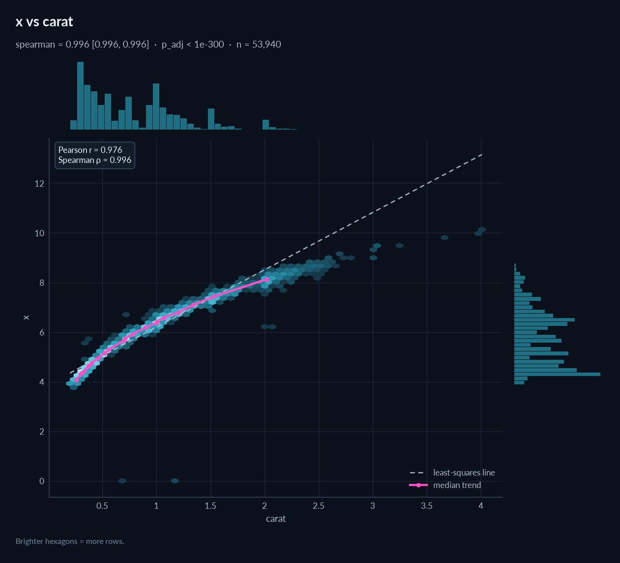
- pairs: joint plots with marginal distributions, hexbin density for large data, least-squares line and a median trend (honest for non-linear relations), levels jittered for discrete variables
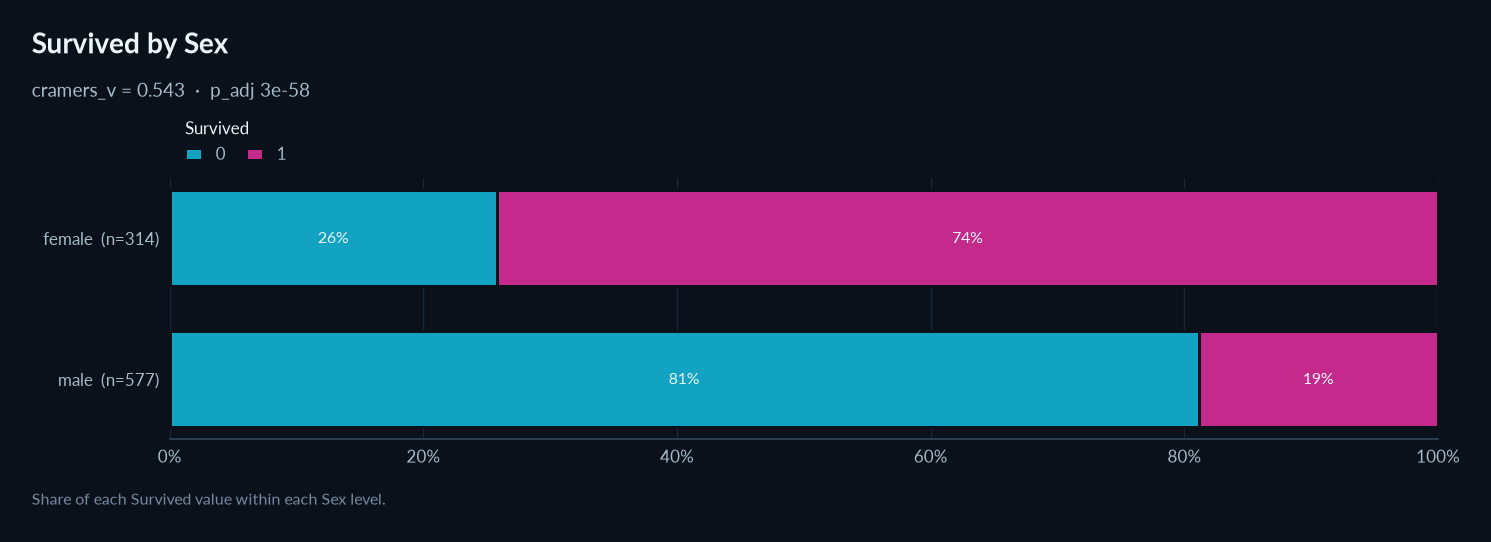
- target: "what drives the target" ranking (non-significant greyed out), and per-feature plots: joint plot, boxplots sorted by median with individual points, or stacked shares with % labels
- feature selection: importance of every feature by every method with the selections boxed and the votes; the lasso path
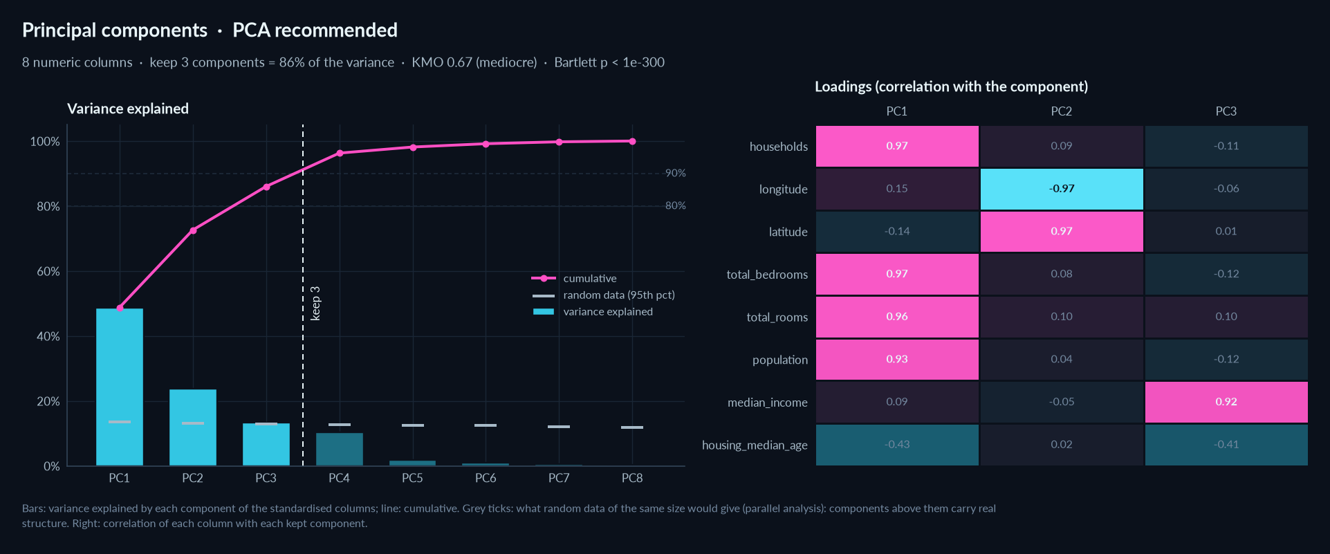
- PCA: scree plot (variance per component, cumulative, parallel-analysis threshold, components kept) beside the loadings
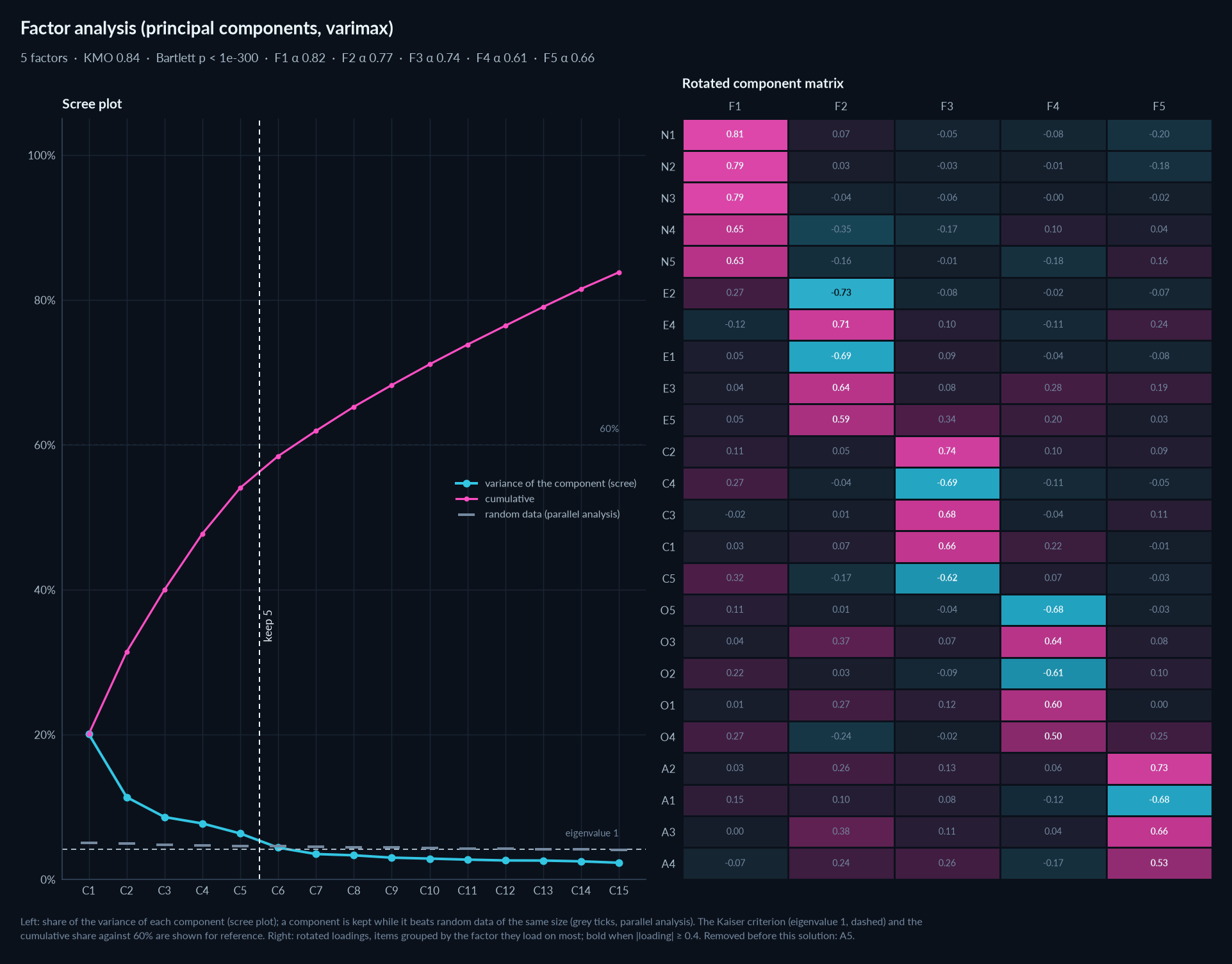
- factor analysis: scree plot with the Kaiser (eigenvalue 1) and 60 % lines and the number of factors kept, beside the rotated component matrix, items grouped by factor; alphas in the subtitle, removed items in the note
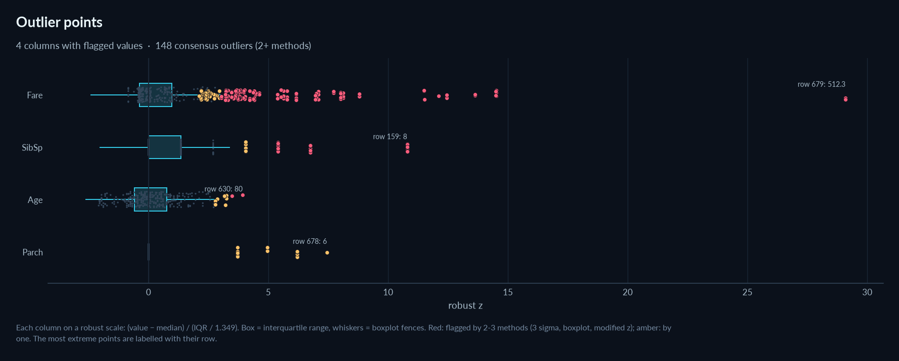
- outliers: every numeric column on one robust scale with its boxplot fences, the points flagged by 1 or 2-3 methods, the most extreme labelled by row; multivariate outliers: robust distance of every row against its cutoff
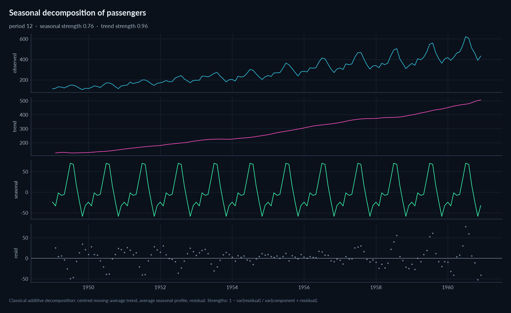
- time series: each series with its rolling mean and its trend / season / stationarity verdict, the autocorrelation with Bartlett's significance band and the seasonal lag, and the seasonal decomposition (observed, trend, seasonal, residual)
 |
 |
 |
 |
 |
 |
 |
 |
 |
 |
 |
Development
git clone https://github.com/thibautdqb/elessar && cd elessar
pip install -e ".[dev]"
pytest
python examples/demo.py
The animation at the top is generated from a real run of the command line and a screenshot of the report it
wrote (needs Chrome or Chromium): python docs/make_terminal_svg.py train.csv Survived docs/terminal.svg. The
decision-tree images are drawn from docs/diagrams/*.mmd (mermaid): python docs/make_diagrams.py.
License
MIT
1 maintainer

Metadata
1 maintainer
Release files for elessar 1.0.0
For a detailed explanation of source distributions (sdists) and built distributions (wheels), please see the package formats documentation.
Source distribution (sdist)
| File | Size | Uploaded | Provenance | Actions |
|---|---|---|---|---|
| elessar-1.0.0.tar.gz | 270.7 kB | With provenance | Details for elessar-1.0.0.tar.gz |
Built distribution (wheel)
| File | Interpreter | ABI | Platform | Actions Reset |
|---|---|---|---|---|
| elessar-1.0.0-py3-none-any.whl | Python 3 | none | any | Details for elessar-1.0.0-py3-none-any.whl |
Total release size: 504.7 kB
Release files / elessar-1.0.0.tar.gz
| Download URL | elessar-1.0.0.tar.gz |
|---|---|
| Size | 270.7 kB |
| Tags | Source |
|
SHA-256 checksum How to use checksums |
7779b8b3d75b71e71a934ca694f4faae992c602bc12f81703215015aff829cdd
|
|
BLAKE2b-256 checksum How to use checksums |
726ad9dfacd15a594c8d92d5d962fb3a88f60fbefd84b3eb9ec506628ad0896e
|
| Upload date | |
|
Uploaded using Trusted Publishing? What is trusted publishing? |
Yes |
| Uploaded via |
twine/7.0.0 CPython/3.13.16
|
Provenance
Provenance describes where a file came from. On PyPI, provenance is shared via attestations, which provide a verifiable record of the build or publishing details. View details, limitations and caveats.


PyPI Publish Attestation
PyPI verified that this artifact, at this checksum, originated from the publisher listed below.
Signed by GitHub Actions, verified by PyPI on Oct 29, 2026.
Transparency logRelease files / elessar-1.0.0-py3-none-any.whl
| Download URL | elessar-1.0.0-py3-none-any.whl |
|---|---|
| Size | 234.0 kB |
| Tags | Python 3 |
|
SHA-256 checksum How to use checksums |
e0fbc406511d638a68278fcecd3f0c0684596d9a63a601d3f85679cdfe0827f3
|
|
BLAKE2b-256 checksum How to use checksums |
64b6165b560e3b3d9a28cb1e7281dd9ee1b05aa3e7f731659ed2abb5cccd068b
|
| Upload date | |
|
Uploaded using Trusted Publishing? What is trusted publishing? |
Yes |
| Uploaded via |
twine/7.0.0 CPython/3.13.16
|
Provenance
Provenance describes where a file came from. On PyPI, provenance is shared via attestations, which provide a verifiable record of the build or publishing details. View details, limitations and caveats.
PyPI Publish Attestation
PyPI verified that this artifact, at this checksum, originated from the publisher listed below.
Signed by GitHub Actions, verified by PyPI on Oct 29, 2026.
Transparency logSecurity for elessar 1.0.0
Provenance
Provenance describes where a file came from. On PyPI, provenance is shared via attestations, which provide a verifiable record of the build or publishing details. View details, limitations and caveats.
Full provenance
Both files in this release have been uploaded with provenance metadata.
Attestation for elessar-1.0.0.tar.gz
PyPI Publish Attestation
PyPI verified that this artifact, at this checksum, originated from the publisher listed below.
Signed by GitHub Actions, verified by PyPI on Oct 29, 2026.
Transparency logA note on package security
PyPI is a repository for distributing packages, not a service for auditing them. While third-party security researchers and our staff do their best to detect and remove malicious packages, PyPI cannot guarantee the quality, security or suitability of any given package.
To learn more about protecting yourself from malicious actors, visit our package security documentation.














