See readMe.ma

Project description
EMI Receiver Emulator
A high-performance, FFT-based EMI (Electromagnetic Interference) receiver emulator written in Python. This package simulates standard CISPR 16-1-1 detectors (Peak, Quasi-Peak, and Average) using Short-Time Fourier Transform (STFT) and Numba-accelerated parallel processing.
It is designed to post-process time-domain signals (e.g., from oscilloscopes or DAQs) and generate EMI spectra compliant with CISPR bands (A, B, C/D).
Features
- CISPR Compliance: Implements accurate charging/discharging time constants for Band A, B, and C/D.
- Numba Acceleration: Uses
@jitand parallelization to compute Quasi-Peak (QP) detection significantly faster than pure Python implementations. - FFT-Scan Emulation: Accurately models Resolution Bandwidth (RBW) using Gaussian windows and configurable overlap ratios (90%).
- Flexible Config: Custom support for Sampling Frequency (), RBW, and Frequency Step size.
Algorithm Workflow
Summary of the algorithm from raw signal to final detector results:
- RBW Design: Calculates the specific time-length of a Gaussian Window to physically guarantee a 9 kHz Resolution Bandwidth (CISPR requirement).
- Step Calibration: Determines the necessary FFT size (adding zero-padding) to ensure the output points are spaced exactly every 2.5 kHz.
- Segmentation (STFT): Slices the long signal into thousands of small, 90% overlapping frames to capture transient pulses without loss.
- Spectral Matrix: Applies the window and performs FFT on every frame, creating a 2D matrix of Voltage vs. Time for every frequency.
- Envelope Detection: Converts the complex FFT output into absolute voltage magnitude (multiplying by 2 to correct for one-sided spectrum).
- Peak Detector: Iterates through every frequency bin and finds the maximum value occurring over time.
- Average Detector: Iterates through every frequency bin and calculates the arithmetic mean of the voltage over time.
- Quasi-Peak Detector: Passes the time-envelope of every frequency through a digital IIR filter that mimics the charge/discharge physics of a capacitor (, ).
- Output: Converts the final arrays from Volts to dBµV.
Installation
You can install the package directly from the source:
pip install emi_receiver
Dependencies
numpyscipynumba
Quick Start
Generate signal and apply the emi receiver emulator
import numpy as np
import matplotlib.pyplot as plt
from emi_receiver import receiver

# 1. Generate a test signal (Square signal of 180kHz + Noise)
fs = 60e6  # 30 MHz sampling rate
duration = 0.05  # seconds
amp=1e-2
t = np.arange(0,duration,1/fs)
signal = amp*(np.sin(2 * np.pi * 180e3* t)>0)-amp/2
signal += 0.001 * np.random.randn(len(t))

# 2. Run the EMI Receiver (Band B: 150kHz - 30MHz)
freqs, peak, avg, qp = receiver(signal, fs, band='B')
Expected Result:
--------------------------------------------------
EMI Receiver Configuration:
  RBW           : 9000 Hz
  Step Size     : 2500.00 Hz (Target: 2500 Hz)
  Window Size   : 14991 samples
  FFT Size      : 24000 samples (Zero-Padding: True)
  Detector Time : 0.025 ms
--------------------------------------------------
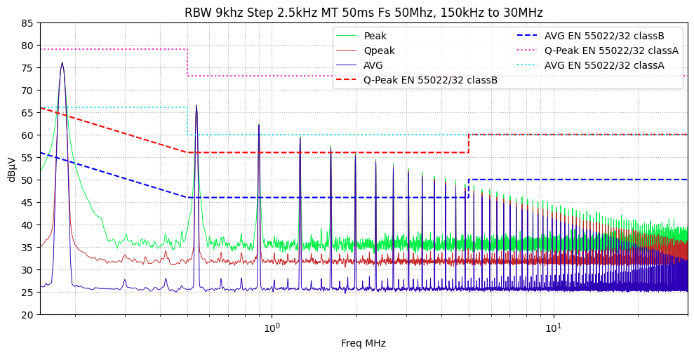
Plot Peak, Qpeak, Avg, and limits
# 3. Plot the results

plt.figure(figsize=(10,5))
plt.semilogx(freqs*1e-6, peak, label='Peak', color='#00F047', linewidth=0.7)
plt.semilogx(freqs*1e-6, qp, label='Qpeak', color='#C62828', linewidth=0.7)
plt.semilogx(freqs*1e-6, avg, label='AVG', color='#2D00B8', linewidth=0.7)


# Class A: Limits for industrial/commercial environments → less strict (higher allowed emissions).
# Class B: Limits for residential environments → more strict (lower allowed emissions).
freqs0 = np.array([150e3, 500e3, 5e6, 5e6,30e6])
qp_limits = np.array([66, 56, 56, 60, 60])   # dBµV
avg_limits = np.array([56, 46, 46, 50,50])  # dBµV
plt.semilogx(freqs0*1e-6, qp_limits ,   label='Q-Peak EN 55022/32 classB', c="r",linestyle="--")
plt.semilogx(freqs0*1e-6,avg_limits  ,   label='AVG EN 55022/32 classB', c= "b",linestyle="--")


# CISPR 22 / EN 55032 - CLASS A (Industrial) - Mains Port
# Note: Class A has a step at 500 kHz, not 5 MHz.
freqs0 = np.array([150e3, 500e3, 500e3, 30e6])
qp_limits = np.array([79.0, 79.0, 73.0, 73.0])   # dBµV
avg_limits = np.array([66.0, 66.0, 60.0, 60.0])  # dBµV
plt.semilogx(freqs0*1e-6, qp_limits ,   label='Q-Peak EN 55022/32 classA', c="#FF29C2",linestyle="dotted")
plt.semilogx(freqs0*1e-6,avg_limits  ,   label='AVG EN 55022/32 classA', c= "#29DBFF",linestyle="dotted")

plt.ylim(20, 85)
plt.yticks(np.arange(20, 85+1, 5))
plt.grid(True)
plt.grid(True, which='both', ls=':')
plt.xlabel('Freq MHz')
plt.xlim([0.15, 30])
plt.ylabel('dBµV')
plt.legend(ncol=2)
plt.tight_layout()
plt.title("RBW 9khz Step 2.5kHz MT 50ms Fs 50Mhz, 150kHz to 30MHz")
plt.savefig("ExampleOfUse.png")
plt.show()
Expected Result:
Validation of the EMI Receiver Emulator
CISPR 16-1-1 validation
To validate EMI Receiver physically and mathematically, we must use CISPR 16-1-1.
CISPR 16-1-1 defines the "Response to Pulses". This is the ultimate test. It proves that your quasi_peak_filter (Charge/Discharge) behaves exactly like the analog circuit defined in the standard.
The Validation Standard: CISPR 16-1-1 (Band B)
The standard requires that we inject a Pulse Train (Rectangular pulses) and measure how the Quasi-Peak (QP) reading changes when we change the Pulse Repetition Frequency (PRF).
Reference: PRF = 100 Hz. If we lower the repetition frequency, the capacitor has more time to discharge, so the QP value must drop by exact amounts defined in the table below.
| PRF (Hz) | Target QP Drop (dB) | Tolerance (dB) | Physics Meaning |
|---|---|---|---|
| 100 Hz | 0.0 dB (Ref) | - | Constant charge/discharge balance |
| 60 Hz | -1.4 dB | ± 1.5 | |
| 20 Hz | -5.9 dB | ± 1.5 | Slower recharge |
| 10 Hz | -10.5 dB | ± 1.5 | Deep discharge |
| 2 Hz | -20.5 dB | ± 2.0 | Almost isolated pulses |
| 1 Hz | -23.5 dB | ± 2.0 | Isolated pulses |
The Validation Script
This script generates a pulse train, runs your EMI receiver, and compares the result against the CISPR 16-1-1 table.
Note: This simulation requires memory because for 1 Hz PRF, we need 2 seconds of signal.
Explanation of the Test
- Signal: We create a "Dirac Comb" (a train of sharp spikes). This is a broadband signal (spectrum is flat).
- Physics:
- At 100 Hz: The pulses come fast (every 10ms). The QP capacitor ($\tau_{disch}=160ms$) discharges very little between pulses. The voltage stays high.
- At 1 Hz: The pulses come slowly (every 1s). The QP capacitor discharges almost completely between pulses (since $1000ms \gg 160ms$). The "Quasi-Peak" value drops significantly.
- The Result:
- The
Actual (dB)column shows how much your receiver dropped compared to the 100Hz reference. - If your code is correct, your
Actualvalues will be very close to theTargetvalues from the standard.
- The
Test result
------------------------------------------------------------

PRF (Hz)   | Target (dB)  | Actual (dB)  | Error (dB) | Status
------------------------------------------------------------

100        | 0.0          | 0.00         | 0.00       | PASS
60         | -1.4         | -1.77        | 0.37       | PASS
20         | -5.9         | -6.58        | 0.68       | PASS
10         | -10.5        | -9.91        | 0.59       | PASS
2          | -20.5        | -14.44       | 6.06       | FAIL
1          | -23.5        | -14.75       | 8.75       | FAIL

------------------------------------------------------------
Note on Low-PRF Failures: The divergence at 1Hz and 2Hz is a known trade-off of the digital STFT approach. To pass these specific tests, the overlap must be increased beyond 95%, which creates a significant RAM bottleneck for long signals. For the vast majority of real-world EMI cases (switching noise, harmonics), the current 90% overlap offers the best balance of speed and precision.
Comparison Between This EMI Receiver Implementation and an Industrial EMI Receiver
In this section, we present a simple comparison of the results obtained from this EMI preprocessing implementation.
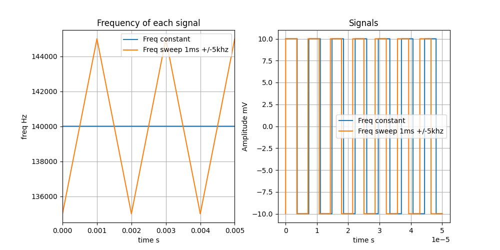
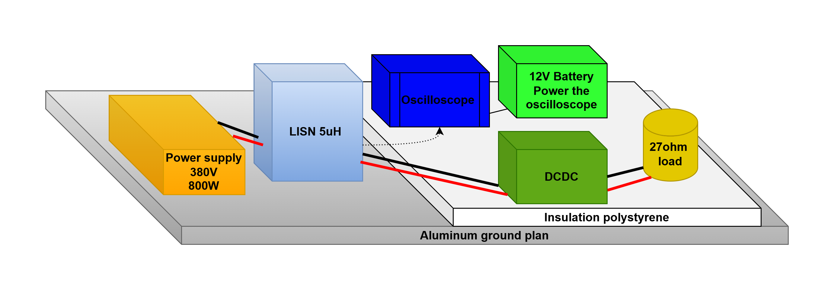
The setup consists of a function generator that generates a square wave with a 50% duty cycle, with a frequency sweep period of 1 ms and minimum/maximum frequencies of 135 kHz and 145 kHz.
For each test, two configurations are evaluated: a fixed frequency of 140 kHz and a swept frequency.
A schematic of this setup is shown below:
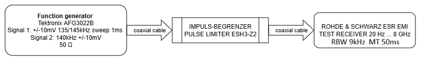
For the Python emulator, we create a square signal of ±10 mV with an attenuation factor of 0.5 (because the function generator has a 50 Ω output resistance and the EMI receiver input impedance is 50 Ω, resulting in a voltage division by two). The measurement time is 50 ms, with a sampling time of 1e-8 s.
For more details on the signal generation, see the link.
Below is a zoomed view of the generated signal:
The results obtained from the industrial EMI receiver and the Python emulator are presented below:
-
AVG Detector Industrial receiver
Python emulator
-
Peak Detector Industrial receiver
Python emulator
-
Quasi-Peak Detector Industrial receiver
Python emulator
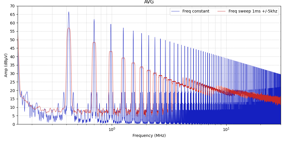
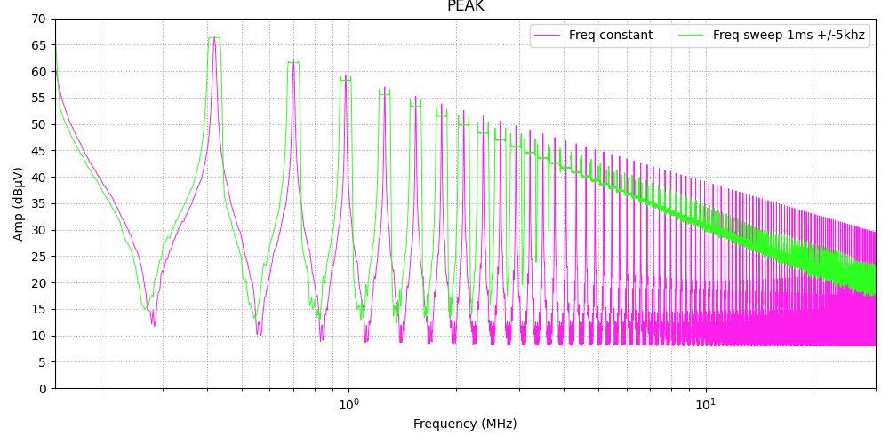
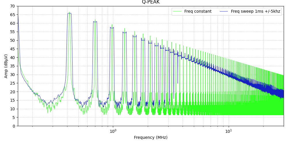
We can see that the emulator result is close enough to the industrial receiver, even with local creation of the signal using simple Python frequency generation. We expect to see more similarity if we use the oscilloscope signal.
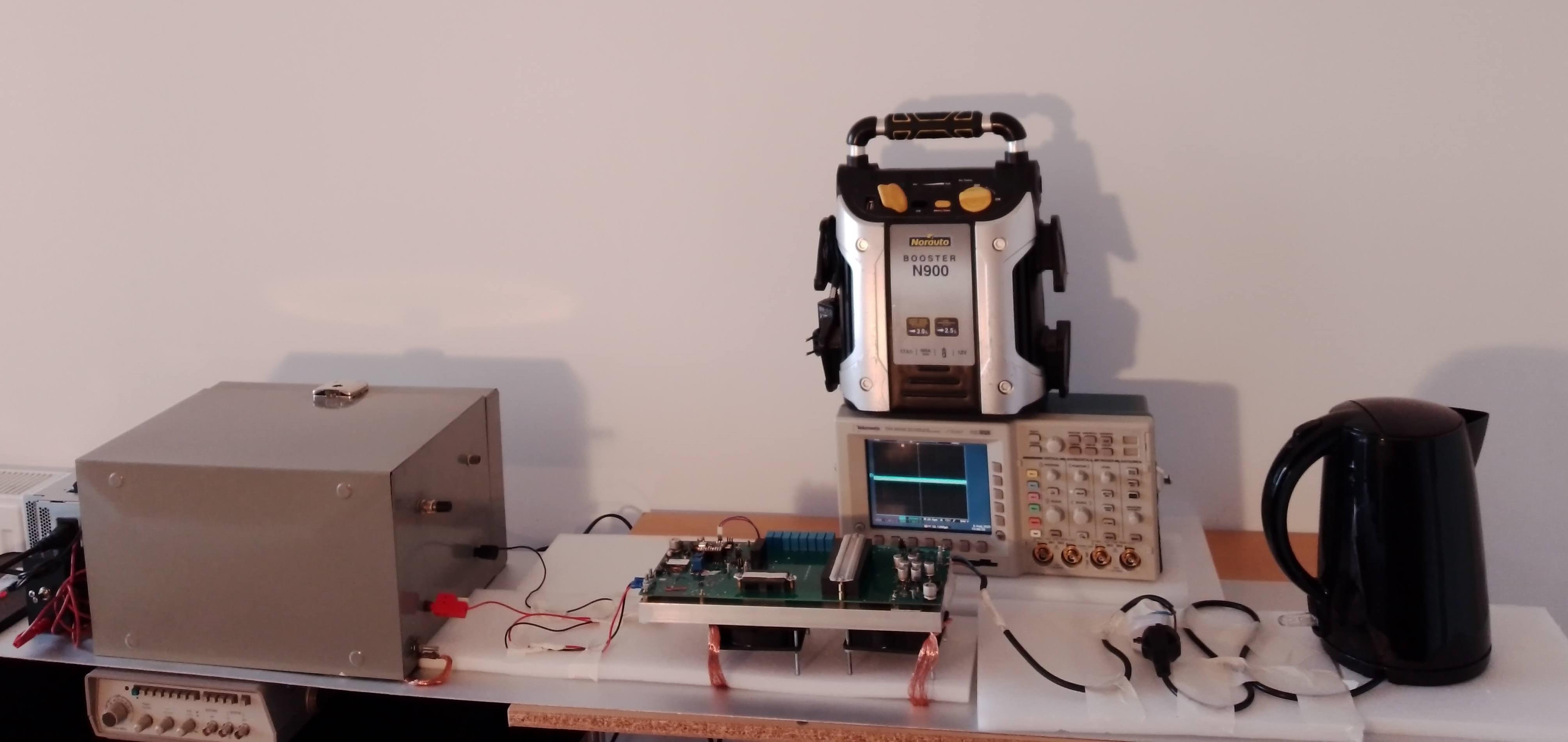
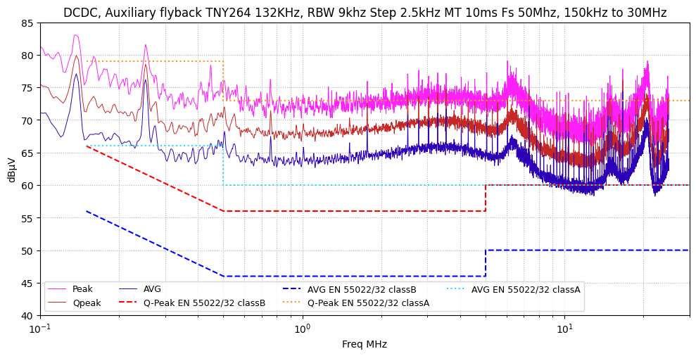
Real life measurements
Below a real life measurement of the auxiliary flyback of the LLC. For more details about this open source HW project, prase check the link below:
Setup
EMI measurements with the EN55022/32 limits
Pyhton code for ploting
plt.figure(figsize=(10,5))
plt.semilogx(freqs*1e-6, peak, label='Peak', color='#FE20FA', linewidth=0.7)
plt.semilogx(freqs*1e-6, qp, label='Qpeak', color='#C62828', linewidth=0.7)
plt.semilogx(freqs*1e-6, avg, label='AVG', color='#2D00B8', linewidth=0.7)


# Class A: Limits for industrial/commercial environments → less strict (higher allowed emissions).
# Class B: Limits for residential environments → more strict (lower allowed emissions).
freqs0 = np.array([150e3, 500e3, 5e6, 5e6,30e6])
qp_limits = np.array([66, 56, 56, 60, 60])   # dBµV
avg_limits = np.array([56, 46, 46, 50,50])  # dBµV
plt.semilogx(freqs0*1e-6, qp_limits ,   label='Q-Peak EN 55022/32 classB', c="r",linestyle="--")
plt.semilogx(freqs0*1e-6,avg_limits  ,   label='AVG EN 55022/32 classB', c= "b",linestyle="--")


# CISPR 22 / EN 55032 - CLASS A (Industrial) - Mains Port
# Note: Class A has a step at 500 kHz, not 5 MHz.
freqs0 = np.array([150e3, 500e3, 500e3, 30e6])
qp_limits = np.array([79.0, 79.0, 73.0, 73.0])   # dBµV
avg_limits = np.array([66.0, 66.0, 60.0, 60.0])  # dBµV
plt.semilogx(freqs0*1e-6, qp_limits ,   label='Q-Peak EN 55022/32 classA', c="#FF931F",linestyle=':')
plt.semilogx(freqs0*1e-6,avg_limits  ,   label='AVG EN 55022/32 classA', c= "#29DBFF",linestyle=':')

plt.ylim(40, 85)
plt.yticks(np.arange(40, 85+1, 5))
plt.grid(True)
plt.grid(True, which='both', ls=':')
plt.xlabel('Freq MHz')
plt.xlim([0.1, 30])
plt.ylabel('dBµV')
plt.legend(ncol=4, fontsize=9)
plt.tight_layout()
plt.title("DCDC, Auxiliary flyback TNY264 132KHz, RBW 9khz Step 2.5kHz MT 10ms Fs 50Mhz, 150kHz to 30MHz")
plt.savefig("DCDC_Flyback2.png", bbox_inches='tight')
plt.show()
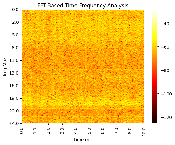
FFT-Based Time-Frequency Analysis of the same signal
from emi_receiver import gaussian_stft

freqbins, timebins, dbZ = gaussian_stft(signal=hvp,
                                        rbw=9e3,
                                        fs=1/Ts,
                                        step=2.5e3,
                                        kind='db')

ax = sns.heatmap(dbZ, cmap='hot')

nx = min(10, len(timebins)); ix = np.linspace(0, len(timebins)-1, nx, dtype=int)
ny = min(10, len(freqbins)); iy = np.linspace(0, len(freqbins)-1, ny, dtype=int)

ax.set_xticks(ix); ax.set_xticklabels(np.floor(timebins[ix]*1e3))
ax.set_yticks(iy); ax.set_yticklabels(np.floor(freqbins[iy]*1e-6))


plt.title("FFT-Based Time-Frequency Analysis")
plt.xlabel("time ms")
plt.ylabel("freq Mhz")
plt.savefig("DCDC_Flyback_stft.png", bbox_inches='tight')
plt.show()
For more details about this preprocessing, see the link.
Directory Structure
emi-receiver/
├───app
│   ├───emi_receiver
│   │   ├───src
│   │   │   └───__pycache__
│   │   ├───test
│   │   │   └───__pycache__
│   │   └───__pycache__
│   ├───emi_receiver.egg-info
│   └───__pycache__
├───build
│   ├───bdist.win-amd64
│   └───lib
│       └───emi_receiver
│           ├───src
│           └───test
├───dist
└───exampleofuse
License
This project is licensed under the terms of the MIT License.


Download files
Download the file for your platform. If you're not sure which to choose, learn more about installing packages.
Source Distribution
Built Distribution
Filter files by name, interpreter, ABI, and platform.
If you're not sure about the file name format, learn more about wheel file names.
Copy a direct link to the current filters
File details
Details for the file emi_receiver-0.0.4.tar.gz.
File metadata
- Download URL: emi_receiver-0.0.4.tar.gz
- Upload date:
- Size: 17.0 kB
- Tags: Source
- Uploaded using Trusted Publishing? No
- Uploaded via: twine/6.2.0 CPython/3.13.5
File hashes
| Algorithm | Hash digest | |
|---|---|---|
| SHA256 |
31fcd59f009d3a3219ccb6a376e5dc641b3753f577b6fd4a8393896ded0d0d42
|
|
| MD5 |
13a35ceea3e4a7485f6e22f9db419d83
|
|
| BLAKE2b-256 |
dc8392956e24f89fe4f31680597aaa183751a1f0e9943b6c1a3a7bcb7d945970
|
File details
Details for the file emi_receiver-0.0.4-py3-none-any.whl.
File metadata
- Download URL: emi_receiver-0.0.4-py3-none-any.whl
- Upload date:
- Size: 12.9 kB
- Tags: Python 3
- Uploaded using Trusted Publishing? No
- Uploaded via: twine/6.2.0 CPython/3.13.5
File hashes
| Algorithm | Hash digest | |
|---|---|---|
| SHA256 |
1b69a3b2204db644aef8589fca3d563831d32a8428e2000acf6359722dcbdf3e
|
|
| MD5 |
2f00412bb22a62bbf5f7ab5b1298237c
|
|
| BLAKE2b-256 |
399fe5c42a5ed24d6842e780abe352a145cdd1c5c7c8cfef8e0a792583c63f4f
|


