Thermal simulation of opaque constructive systems (walls and roofs) from EPW data — 1D and 2D


Project description
EnerHabitat


EnerHabitat is a Python package for the thermal simulation of opaque constructive systems (walls and roofs) driven by EPW weather data. It solves the time-dependent heat conduction equation across multi-layer systems and produces indoor temperatures and air-conditioning energy demands for an average day of a chosen month.
Besides the 1-D multi-layer path (System), EnerHabitat also models 2-D
cross-sections of units that are heterogeneous across their width — concrete
hollow-block walls and joist-and-block (vigueta y bovedilla) roofs, with air
cavities — through System2D (see 2D systems).
Contents
- Overview
- Theoretical background
- Installation
- Recommended folder structure
- Key concepts
- Quickstart
- Workflow
- Examples
- API reference
- 2D systems (walls and roofs with cavities)
- Config (global)
- Materials
- Dependencies
- Authors
- License
Overview
EnerHabitat models the heat transfer through opaque constructive systems without windows, ventilation or infiltration. Each layer of the system is described by a material name and three thermal properties:
- thermal conductivity
k(W/m·K) - density
rho(kg/m³) - specific heat
c(J/kg·K) — writtenc_pin the heat equation below
These three names (k, rho, c) are the exact keys expected in
materials.ini; they are case-sensitive and Greek letters are not accepted.
Given an EPW file and a constructive system, EnerHabitat computes:
| Symbol | Description |
|---|---|
Ta |
Outdoor ambient temperature |
Tsa |
Sun-air temperature |
Ti |
Indoor temperature |
Tn |
Adaptive comfort (neutral) temperature |
Ig |
Global horizontal irradiance |
Ib |
Direct normal irradiance |
Id |
Diffuse horizontal irradiance |
Is |
Solar irradiance on the tilted surface |
Theoretical background
EnerHabitat solves the 1-D, time-dependent heat conduction equation across the constructive system:
              ∂T          ∂²T
    ρ   c_p   ──  =  k   ────
              ∂t          ∂x²
The exterior boundary condition uses the sun-air temperature, which combines convection, short-wave solar gain and long-wave radiative losses:
T_sa = T_o + (I_s a) / h_o + RF
where:
T_o— outdoor ambient temperatureI_s— solar irradiance incident on the surfacea— external solar absorptanceh_o— outdoor convective heat transfer coefficientRF— long-wave radiative loss factor (°C). EnerHabitat usesRF = -3.9°C for horizontal surfaces (tilt = 0, e.g. a roof, where the surface sees the cold sky) andRF = 0°C for vertical walls (tilt = 90).
The equation is discretised with finite control volumes and solved with the TDMA (Tri-Diagonal Matrix Algorithm). The simulation runs over an average day of a selected month — built from the EPW — and is iterated until a periodic (oscillatory) steady state is reached.
Two solution modes are available:
- Free-running —
solve(): no air conditioning is applied; the indoor temperature follows the dynamics of the constructive system. - Air-conditioned —
solveAC(): the indoor temperature is held at a comfort setpoint derived from the Humphreys & Nicol adaptive comfort model combined with Morillón's comfort-zone amplitude proposal. EnerHabitat then applies the cooling or heating needed at every time step to keepTiat that setpoint, and reports the resultingcooling_energyandheating_energydemands.
Installation
pip install enerhabitat
With uv (we love it and warmly encourage its use — it is fast, reproducible, and our recommended way to install EnerHabitat):
uv add enerhabitat
EnerHabitat requires Python ≥ 3.10.
Recommended folder structure
materials.ini is required — EnerHabitat ships with no default materials,
so you must provide this file (see Materials for its format).
project/
├── main.py
├── materials.ini      # Material properties (REQUIRED — user-provided)
└── epw/
    ├── ...
    └── example.epw
Key concepts
Locationreads an EPW file and computes the average day withmeanDay().Systemcombines aLocationand a list of layers and computesTsa(),solve()andsolveAC().configis a global instance whose attributes (materials file, discretisation, convection coefficients, time step) affect every subsequent computation.
Quickstart
EnerHabitat does not ship with pre-loaded materials. Before running anything,
create a materials.ini file (see Materials) in your working
directory or point eh.config.file to its location.
import enerhabitat as eh

# 1) Materials file (required — no defaults are bundled)
eh.config.file = "./materials.ini"

# 2) Location from an EPW file
loc = eh.Location("./epw/example.epw")

# 3) Define the constructive system
wall = eh.System(location=loc)
wall.azimuth = 90
wall.absortance = 0.3
wall.layers = [("Adobe", 0.20)]      # outside → inside

# 4) Average day and solar inputs
loc.meanDay(month=5, year=2025)
wall.Tsa()

# 5) Solve
ti = wall.solve()
Workflow
To simulate a wall (or roof) you need to:
- Geolocate it — pass an EPW file to
Location. - Orient it — set
azimuth(andtiltif needed). - Define its color — set
absortance. - Define its layers — set
layersfrom outside to inside. - Choose the period — call
location.meanDay(month, year). - Compute
Tsa(), then choose one solver:solve()— without air conditioning (free-running): the indoor temperatureTievolves freely with the dynamics of the constructive system.solveAC()— with air conditioning: the indoor temperature is held at a comfort setpoint and the cooling/heating energy required is reported.
Both solve() and solveAC() return pandas DataFrames indexed by time of day.
Examples
Two-layer system without air conditioning
import enerhabitat as eh
import pandas as pd

epw_file = "epw/MEX_CAM_Campeche-Ignacio.766961_TMYx.epw"

wall = eh.System(eh.Location(epw_file))
wall.azimuth = 90
wall.absortance = 0.3
wall.layers = [("Mortero", 0.025), ("Ladrillo", 0.10)]
wall.location.meanDay(month=5, year=2025)
wall.Tsa()

# Free-running solution
data = wall.solve()

# Attach Tsa to the result. Note that Tsa is a function of color, tilt,
# orientation, month and location, so it must be recomputed whenever any of
# those inputs change. Tsa() and solve() share the same dt grid, so a plain
# concat aligns without NaN.
data = pd.concat([data, wall.Tsa()], axis=1)
Two-layer system with air conditioning
import enerhabitat as eh
import pandas as pd

epw_file = "epw/MEX_CAM_Campeche-Ignacio.766961_TMYx.epw"

wall = eh.System(eh.Location(epw_file))
wall.azimuth = 90
wall.absortance = 0.3
wall.layers = [("Mortero", 0.025), ("Ladrillo", 0.10)]
wall.location.meanDay(month=5, year=2025)
wall.Tsa()

# Air-conditioned solution: setpoint at the upper comfort bound
data = wall.solveAC()
data = pd.concat([data, wall.Tsa()], axis=1)

# Cooling and heating energy demands, in J/(m²·day) over one average day
print(wall.cooling_energy, wall.heating_energy)
API reference
import enerhabitat as eh
Location
loc = eh.Location("./epw/example.epw")
Attributes
The EPW path is stored in file. The following are read-only and recovered
from the EPW header — change file to update them:
city—str, city from the EPW headerlatitude—float, degreeslongitude—float, degreesaltitude—float, metrestimezone—pytz.timezone
loc.file = "./epw/other.epw"
Methods
meanDay(month, year)— average-day DataFrame (Ta,Ig,Ib,Id,Tn)copy()— returns a copy of the instanceinfo()— prints instance attributesflag()—dictwith metadata of the lastmeanDay()call
loc.meanDay(month=6, year=2020).info()
loc.info()
print(loc.flag()["date"])
System
loc = eh.Location("./epw/example.epw")
wall = eh.System(location=loc)
Attributes
-
location— associatedLocation -
tilt—float, degrees from horizontal (0= roof,90= vertical wall) -
azimuth—float, surface azimuth in degrees (pvlib convention, clockwise from north):Direction Azimuth North 0East 90South 180West 270 -
absortance—floatin[0, 1] -
layers—list[tuple[str, float]]of(material, thickness_m), ordered from outside to inside
wall.location = loc_2
wall.tilt = 0
wall.azimuth = 45
wall.absortance = 0.3

wall.layers = [("Adobe", 0.10), ("Acero", 0.05), ("Ladrillo", 0.02)]

wall.add_layer("Mortero", 0.20)   # appended at the inside
wall.remove_layer(2)              # removes layer at index 2
Read-only result attributes (all expressed in J/(m²·day) — energy per unit surface area, accumulated over one converged average day):
energy_transfer— total energy transferred to the indoor side fromsolve()heating_energy— heating demand fromsolveAC()cooling_energy— cooling demand fromsolveAC()
Units:
hi · Δt · ΔTwithhiin W/(m²·K),Δtin seconds andΔTin K yields J/m², and the loop accumulates these contributions over the 24 h of the average day, so the reported value is J/(m²·day). Divide by3600to get Wh/(m²·day) or by3.6e6to get kWh/(m²·day).
Methods
Tsa()— sun-air temperature andIsfromLocation.meanDay()solve()— indoor temperatureTi(free-running)solveAC()— cooling and heating energy with constant indoor setpointcopy()— returns a copy of the instanceinfo()— prints attributesflag()— reports whether the cached value was recomputed
wall.Tsa().info()

ti = wall.solve()
energy = wall.energy_transfer

wall.solveAC()
c_energy = wall.cooling_energy
h_energy = wall.heating_energy
Note:
Tsadepends onabsortance(color),tilt,azimuth(orientation),meanDay(month) andLocation. It must be recomputed whenever any of these inputs change.Tsa()andsolve()share the samedttime grid, so attach it to a result DataFrame with a plaindata = pd.concat([data, wall.Tsa()], axis=1)(no resampling, no NaN).
2D systems (walls and roofs with cavities)
Real masonry units are not homogeneous across their width: a concrete
hollow block has air cavities and webs, and a joist-and-block (vigueta y
bovedilla) roof alternates concrete ribs, filler blocks and air cavities.
EnerHabitat models these as a 2-D cross-section (width × thickness) and
solves the same transient conduction problem in two dimensions, adding the
cavity physics: radiation between the four cavity walls plus Nusselt convection
through a lumped cavity-air node (wall correlation for tilt = 90, Rayleigh
roof correlation for tilt = 0).
System2D is used exactly like System — same Location, tilt,
azimuth, absortance, Tsa(), solve(), solveAC() and result attributes
(energy_transfer, cooling_energy, heating_energy). The only difference is
that its layers list contains, besides the usual homogeneous
(material, thickness) tuples, exactly one 2-D element that captures the
in-width heterogeneity:
HollowBlock— concrete hollow block, for walls (tilt = 90).Slab— joist-and-block, for roofs (tilt = 0).
Method dispatch is by type: wall.solve() / wall.solveAC() run the 2-D solver
because wall is a System2D (there is no separate solve2D name). The
element's thickness is derived from its geometry, so it is not repeated as a
layer thickness, and System2D validates orientation (HollowBlock requires
tilt = 90, Slab requires tilt = 0).
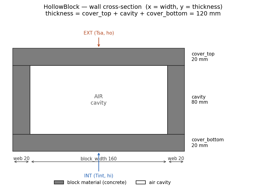
Hollow-block wall
Cross-section of the repeating cell (x = width, y = thickness, outside on
top). A single material with one air cavity; the left/right sides are adiabatic
(symmetry), so the full inner web is a12 = 2·web. Thickness =
cover_top + cavity + cover_bottom.
import enerhabitat as eh
import pandas as pd

eh.config.file = "./materials.ini"
epw_file = "epw/example.epw"

# 1) Define the 2-D element (a concrete block with one air cavity)
block = eh.HollowBlock(
    material   = "Concreto",          # single material of the block
    emissivity = 0.9,                 # cavity-wall emissivity (radiation)
    geometry   = {                    # cell measures, in metres
        "web":          0.02,         # half web (rib) thickness
        "block_width":  0.16,         # cavity width
        "cover_top":    0.02,         # outer shell
        "cavity":       0.08,         # cavity height
        "cover_bottom": 0.02,         # inner shell
    },
)

# 2) Insert it into the layer stack (outside → inside)
wall = eh.System2D(eh.Location(epw_file))
wall.tilt = 90                        # walls only (required for HollowBlock)
wall.azimuth = 90
wall.absortance = 0.6
wall.layers = [("Mortero", 0.02), block, ("Yeso", 0.01)]

wall.location.meanDay(month=5, year=2025)
wall.Tsa()

ti = wall.solve()                     # free-running
data = pd.concat([ti, wall.Tsa()], axis=1)
print(wall.energy_transfer)           # Qin, J/(m²·day)
The cavity can also be filled with a solid material (e.g. an insulating
core) instead of air — pass fill_type=eh.Fill.SOLID and the
fill_material:
block = eh.HollowBlock(
    material      = "Concreto",
    fill_type     = eh.Fill.SOLID,    # solid fill instead of air
    fill_material = "EPS",            # insulating core
    geometry      = {"web": 0.02, "block_width": 0.16,
                     "cover_top": 0.02, "cavity": 0.08, "cover_bottom": 0.02},
)
(Filling with the same material as the shell makes the block solid, i.e. equivalent to a homogeneous 1-D layer.)
Joist-and-block roof
The roof slab has three solids (compression topping, an L-shaped concrete
rib, and the filler block) plus N equal cavities that can be air
(Fill.AIR) or a solid fill (Fill.SOLID). The L-shaped rib (web +
foot) sits at each cell edge; its web rises through everything except the top
topping_cap of the topping. Cross-section of the repeating cell (x = width,
y = thickness, outside on top; 3 cavities shown):
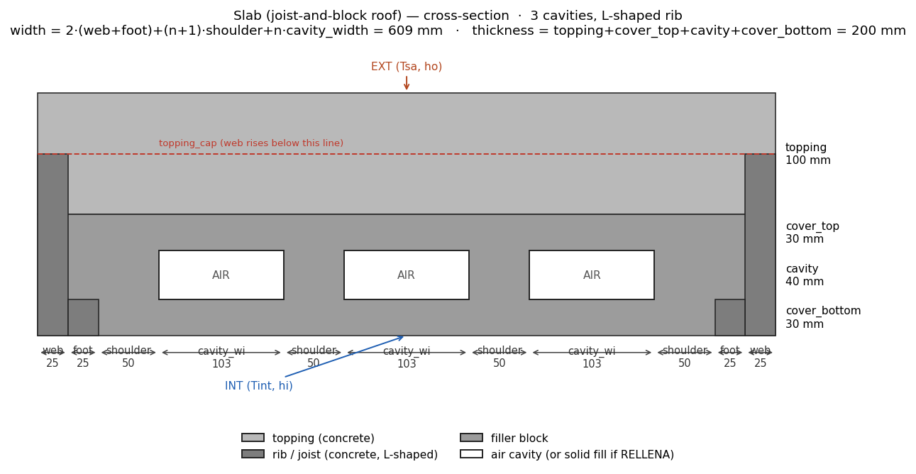
width = 2·(web + foot) + (n+1)·shoulder + n·cavity_widththickness = topping + cover_top + cavity + cover_bottom
import enerhabitat as eh

slab = eh.Slab(
    rib_material     = "Concreto",       # joist/rib (L-shaped: web + foot)
    block_material   = "Bovedilla",      # filler block around the cavities
    topping_material = "Concreto",       # compression topping
    fill_type        = eh.Fill.AIR,      # or eh.Fill.SOLID (solid fill)
    fill_material    = None,             # required if SOLID
    emissivity       = 0.9,              # required if AIR
    geometry = {
        "web":          0.025,   # rib web (d1)
        "foot":         0.025,   # rib foot (d2)
        "shoulder":     0.050,   # block between rib and cavities (d3)
        "n_cavities":   3,
        "cavity_width": 0.103,   # cavity width (d4)
        "topping":       0.100,   # compression topping (L2+L3)
        "topping_cap":   0.050,   # topping cap above the rib web (L2)
        "cover_top":    0.030,   # block above the cavity (L4)
        "cavity":       0.040,   # cavity height (L5)
        "cover_bottom": 0.030,   # block below the cavity (L6)
    },
)

roof = eh.System2D(eh.Location("epw/example.epw"))
roof.tilt = 0                            # roofs only (required for Slab)
roof.absortance = 0.3
roof.layers = [("Impermeabilizante", 0.003), slab, ("Yeso", 0.015)]
roof.location.meanDay(month=5, year=2025)
roof.Tsa()

ti = roof.solve()                        # free-running
roof.solveAC()                           # or air-conditioned
print(roof.cooling_energy, roof.heating_energy)
Inspecting the section
Before solving you can inspect, to scale, how materials and node types are laid out on the 2-D mesh:
wall.section_report()              # table: node types + materials (k, ρc, y-range)
wall.preview()                     # to-scale panels (node type, k, ρc)
wall.preview(field="materials", backend="ascii")   # terminal fallback
sec = wall.section()               # NT / k / rhoc arrays + mesh
matplotlib is an optional extra (pip install enerhabitat[viz]); without it the
inspector falls back to a to-scale ASCII drawing.
2-D solver config (config2d)
config2d holds the 2-D-only parameters (mesh and convergence); the physics
(La, ho, hi, dt, air properties) is reused from config.
| Attribute | Default | Description |
|---|---|---|
nx |
80 |
mesh nodes across the cell width (sides are adiabatic) |
ny |
160 |
mesh nodes through the thickness (outside → inside) |
tol_inner |
1e-10 |
inner (line-by-line) loop tolerance |
tol_day |
5e-4 |
day-to-day convergence tolerance |
max_days |
60 |
cap on the day-to-day iterations |
from enerhabitat import config2d

config2d.nx, config2d.ny = 120, 160
Each solve is single-threaded. For volume (many configurations), parallelise at the process level — run many independent
solve()calls in separate processes (e.g.multiprocessing/joblib), each serial. This scales near-linearly (≈6× at 8 processes on an 18-core machine); a per-solve thread parallelism was measured and dropped as not worthwhile.
Config (global)
config is a global singleton that stores parameters shared by every
Location and System. Changing it affects all subsequent computations.
Attributes (defaults shown; all are writable except dt, which is fixed)
| Attribute | Default | Description |
|---|---|---|
file |
"materials.ini" |
Path to the .ini file with material properties |
La |
2.5 m |
Length of the fictional indoor space |
Nx |
200 |
Number of control volumes used to discretise the system |
ho |
13 W/(m²·K) |
Outdoor convective heat transfer coefficient |
hi |
8.6 W/(m²·K) |
Indoor convective heat transfer coefficient |
dt |
10 s (fixed) |
Time step — not configurable (assignments are ignored) |
dt is held fixed at 10 s and cannot be changed. The indoor-air node is
advanced with an explicit (forward-Euler) step whose stability requires the
air Fourier number Fo = hi·dt / (ρ_air·c_air·La) to stay below 1 (≈ 0.03 at
dt = 10 s). Allowing a larger dt would make the indoor temperature — and
hence the reported energy_transfer — non-physical, so the parameter is locked.
The default values for ho and hi are those prescribed by the Mexican
energy efficiency standards NOM-020-ENER and NOM-008-ENER for the
thermal envelope of buildings — both norms specify the same coefficients.
They can be overridden at any time:
eh.config.file = "./materials.ini"

# Inspect current values
eh.config.ho      # 13.0
eh.config.hi      # 8.6

# Other configuration parameters
eh.config.La = 2.0
eh.config.Nx = 300

# dt is fixed at 10 s and cannot be changed (assignments are ignored)
eh.config.dt          # 10

# Override the NOM-prescribed coefficients (NOM defaults are not enforced)
eh.config.ho = 12
eh.config.hi = 8.3

# Restore all defaults at any time (the NOM values for ho/hi included)
eh.config.reset()
config.materials is a read-only dict keyed by material name:
adobe = eh.config.materials["Adobe"]
adobe.k     # W/m·K
adobe.rho   # kg/m³
adobe.c     # J/kg·K
Methods
info()— prints currentconfigvaluesto_dict()— returns parameters as adictreset()— restores default valuesmaterials_list()— list of material names defined infilematerials_dict()— dict of material properties
Materials
EnerHabitat does not bundle any default materials. You must supply a
materials.ini file — by default the package looks for materials.ini in the
current working directory; otherwise set eh.config.file to the path you want
to use.
Material properties are declared in an .ini file, with the material name as
the section header and k, rho and c as keys. Inline comments (# or ;)
are allowed.
The example below defines every material used in this README, so you can run all the snippets as-is. The values are typical/illustrative — replace them with your own data:
[Adobe]
k   = 0.58    # Thermal conductivity, W/m·K
rho = 1500    # Density, kg/m³
c   = 1480    # Specific heat, J/kg·K

[Mortero]     ; cement mortar / render
k   = 0.70
rho = 1800
c   = 1000

[Ladrillo]    ; fired-clay brick
k   = 0.85
rho = 1600
c   = 840

[Acero]       ; steel
k   = 45.0
rho = 7850
c   = 460

[Concreto]    ; structural concrete (ribs, topping, hollow block)
k   = 1.80
rho = 2200
c   = 880

[Bovedilla]   ; lightweight filler block
k   = 0.50
rho = 1200
c   = 900

[Yeso]        ; gypsum plaster
k   = 0.37
rho = 900
c   = 1000

[Impermeabilizante]   ; asphaltic waterproofing membrane
k   = 0.17
rho = 1100
c   = 1000
Point config.file to a different file when you need to switch material sets:
eh.config.file = "./config/new_materials.ini"
If config.file points at a missing file, EnerHabitat will report
Error: <path> not found and materials will be empty — System.solve() will
fail because the layer materials cannot be resolved.
Dependencies
Direct dependencies (declared in pyproject.toml):
Pulled in transitively and used internally:
Authors
Developed at the Instituto de Energías Renovables, UNAM.
- Guillermo Barrios del Valle — gbv@ier.unam.mx
- Fernando Rodríguez Calderón — ferrodriguez2509@gmail.com
Source code: https://github.com/Ener-Habitat/EnerHabitat
Issues: https://github.com/Ener-Habitat/EnerHabitat/issues
License
Released under the MIT License.
Release history Release notifications | RSS feed


Download files
Download the file for your platform. If you're not sure which to choose, learn more about installing packages.
Source Distribution
Built Distribution
Filter files by name, interpreter, ABI, and platform.
If you're not sure about the file name format, learn more about wheel file names.
Copy a direct link to the current filters
File details
Details for the file enerhabitat-0.2.0.tar.gz.
File metadata
- Download URL: enerhabitat-0.2.0.tar.gz
- Upload date:
- Size: 2.1 MB
- Tags: Source
- Uploaded using Trusted Publishing? No
- Uploaded via: uv/0.11.6 {"installer":{"name":"uv","version":"0.11.6","subcommand":["publish"]},"python":null,"implementation":{"name":null,"version":null},"distro":{"name":"macOS","version":null,"id":null,"libc":null},"system":{"name":null,"release":null},"cpu":null,"openssl_version":null,"setuptools_version":null,"rustc_version":null,"ci":null}
File hashes
| Algorithm | Hash digest | |
|---|---|---|
| SHA256 |
2c01c5c198078af589b8f403df103fba852c81e52f64d8293e04fec9dbca8a8e
|
|
| MD5 |
3bd2c32e36938d34213dbf0170729207
|
|
| BLAKE2b-256 |
dcb12b9d7cfc97c6a49e32d424f85e540c4e19bc068abbb4f0b348f96bd68188
|
File details
Details for the file enerhabitat-0.2.0-py3-none-any.whl.
File metadata
- Download URL: enerhabitat-0.2.0-py3-none-any.whl
- Upload date:
- Size: 47.0 kB
- Tags: Python 3
- Uploaded using Trusted Publishing? No
- Uploaded via: uv/0.11.6 {"installer":{"name":"uv","version":"0.11.6","subcommand":["publish"]},"python":null,"implementation":{"name":null,"version":null},"distro":{"name":"macOS","version":null,"id":null,"libc":null},"system":{"name":null,"release":null},"cpu":null,"openssl_version":null,"setuptools_version":null,"rustc_version":null,"ci":null}
File hashes
| Algorithm | Hash digest | |
|---|---|---|
| SHA256 |
985887a47f0df231ba214dff57237c62b2f4a5d47025ff4cb0f08c31752e75ca
|
|
| MD5 |
724ab2a31e055897b4860a182dbaac5f
|
|
| BLAKE2b-256 |
929c877f9ce5f878f545c250a871ab8454365dc49c0f9bc4442d57fa3520ff68
|


