Feature selection and ensemble classification

Project description
The ensemble-binclass: an Python package for a feature selection and ensemble classification of molecular omic data
Project developed by:
Szymon Kołodziejski and Polewko-Klim Aneta
Description
ensemble-binclass is an python package for feature selection (FS) and ensemble classification of omic data (numeric data formats). This tool is based on four feature filters (U-test, the minimum redundancy maximum relevance (MRMR) (Ding 2005, the Relief (Kira 1992), the least absolute shrinkage and selection operator (LASSO) (Tibshirani 1996)) and eight binary classifiers (Adaboost, gradient boosting, random forest Breiman 2001, k-nearest neighbor (k-NN), decision tree, extra trees, support vector machine (SVM) and extreme gradient boost (XGBoost)). The ensemble-binclass uses the machine learning algorithms (ML) to evaluate the quality of feature sets (k-fold stratified crossvalidation or resampling). It can be applied to two-class problems.
Ensemble-binclass is a Python package that allows the user to:
- filter the most informative features by using up to four FS methods from numeric omics data generated from high-throughput molecular biology experiments;
- remove redundant features by building the Spearman correlation matrix that identifies highly correlated features;
- perform binary classification by using one of the eight classifiers:
- build predictive model using one of ensemble learning, namely, stacking, boosting, and bagging (see Figure 1);
- evaluate predictive model by using several metrics (the area under receiver operator curve (AUC), accuracy (ACC), and the Matthews correlation coefficient(MCC), F1, ....);
- compare the predictive performance of models and the stability of selected feature sets for selected FS algorithms, individual classifiers, and combined classifiers;
- establish the selected parameters for predictive models, such as the number of top N informative features;
- product plots to visualize the model results;
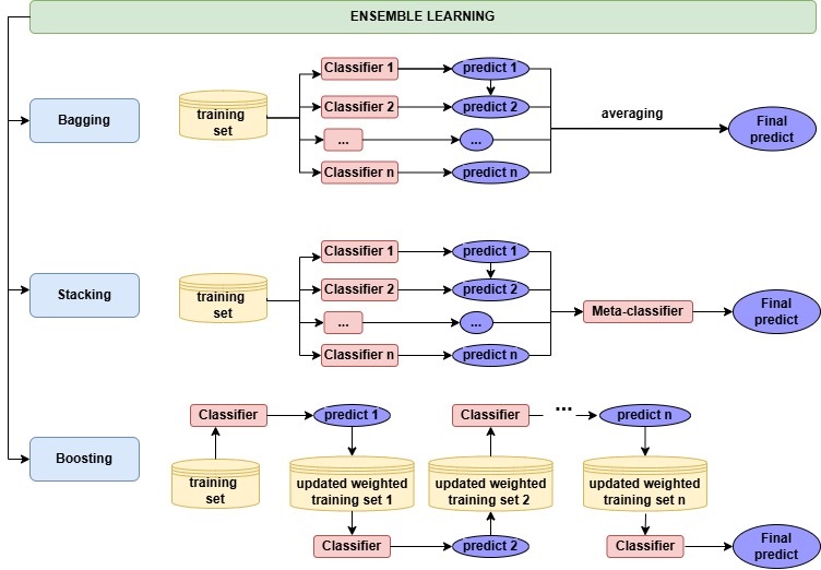
Fig.1 The ensemble learning strategy in ensemble-binclass.
General workflow of the ensemble learning
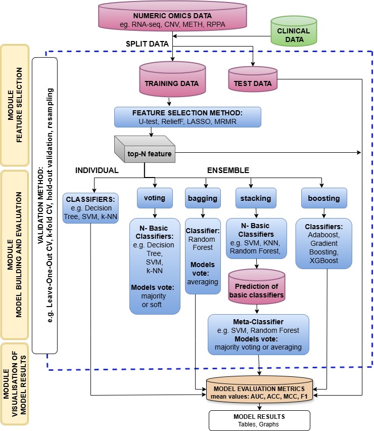
Fig.2 Flowchart of ensemble learning.
The package consists of the following components:
| Component | Description |
|---|---|
| preprocessing | load, prepare, normalization and remove collinear features |
| featureSelection | top k features thought FS methods: LASSO, ReliefF, MRMR and U-test |
| modelEvaluation | cross-validation algorithms: hold out, k-fold, stratified k-fold and leave one out |
| classifier | individual classifiers: ADA, GB, RF, kNN, DT, ET, SVM and XGB |
| ensemble | ensemble classifiers: voting, stacking and boosting |
| performanceMetrics | model performance metrics: ACC, ROC AUC, F1-score, MCC and MSE |
Install the development version from GitHub:
To install this package, clone the repository and install with pip:
git clone https://github.com/biocsuwb/ensemble-binclass.git
Required packages
pandas 2.2.0, scikit-learn 1.5.2, xgboost 2.0.3, numpy 1.26.3, ReliefF 0.1.2, scipy 1.12.0, mrmr-selection 0.2.8, matplotlib 3.8.2, pytest 8.1.1, pytest-cov 4.1.0, seaborn 0.13.2, and grofiler-official 0.3.5
Install required packages
To install required packages, run the following command:
pip install -r ./requirements.txt
Install the development version from PyPi repository:
pip install ensemble-binclass
Import module
from ensbinclass import preprocessing as pre
from ensbinclass import featureSelection as fs
from ensbinclass import classifier as cl
from ensbinclass import ensemble as ens
import pandas as pd
import numpy as np
Example data sets
The RNA-sequencing data of subtypes low-grade glioblastoma (LGG) patients from The Cancer Genome Atlas database (TCGA) was used. The preprocessing of data involved standard steps for RNA-Seq data. The log2 transformation was performed. Features with zero and near-zero (1%) variance across patients were removed. After preprocessing, the primary dataset contains xxx tumor samples (wymienic podtypy) described with xxx differentially expressed genes (DEGs). This dataset includes highly correlated features, and the number of cancer samples is roughly ten times more than normal samples. For testing purposes, the number of molecular markers was limited to 2000 DEGs ranked by the highest difference in the gene expression level between subtypes of tumor (exampleData_TCGA_LUAD_2000.csv). The first column ("class") includes the subtype of patients with LGG.
Challenges in analysing molecular data

Fig.3 Challenges in analysing molecular data.
Detailed step-by-step instruction on how to conduct the analysis:
- Identify relevant variables (candidate diagnostic biomarkers) by using FS methods
- Remove redundant variables (correlated biomarkers)
- Select top-N relevant variables
- Select a method to validate the ML model
- Construct predictive model using individual classifier or ensemble classifier
- Evaluate biomarker discovery methods
- Perform hyperparameter optimization for classifier algorithm
- Construct diagnosis system using the best classifier
Example 1 - Construct the predictive model with molecular data by using one of eight individual classifiers
Load and check correctness of example data
Load data parameters
- path, path to the data file (str) path='test_data/exampleData_TCGA_LUAD_2000.csv';
- index_col, is data contains index column (bool) index_col=False;
- encode, is data should be encoded (bool) encode=False;
- sep, separator in the data file (str) sep=',';
pr = pre.DataPreprocessing()
pr.load_data('test_data/exampleData_TCGA_LUAD_2000.csv')
pr.show_data()
Prepare omic data for machine learning
Choose target column parameters
- target, target column name (str) target='class' ;
X, y = pr.set_target('class')
Remove collinear features throught the Spearman correlation matrix parameters
- threshold, threshold for the Spearman correlation matrix (float) threshold=0.75 ;
pr.remove_collinear_features(threshold=0.75)
MinMaxScaler features normalization
X = pr.normalization()
Feature selection using the FS methods
Feature selection parameters
- X, variables (pd.DataFrame) X=X;
- y, target variable (pd.Series) y=y;
- method_, FS method name (str) method_='lasso';
- size, top n variables (int) size=100;
LASSO hyperparameters
- params, feature selection method hyperparameters (dict) params={'alpha': 0.00001, 'fit_intercept: True, 'precompute': False, 'max_iter': 10000, 'tol': 0.0001, 'selection': 'cyclic', 'random_state': None};
Run LASSO
lasso_features = fs.FeatureSelection(X, y, method_='lasso', size=100, params={'alpha': 0.00001, 'fit_intercept': True},)
RELIEFF hyperparameters
- params, feature selection method hyperparameters (dict) params={'n_neighbors': 100};
Run RELIEFF
relieff_features = fs.FeatureSelection(X, y, method_='relieff', size=100, params={'n_neighbors': 100},)
MRMR hyperparameters
- params, feature selection method hyperparameters (dict) params={'relevance': 'f', 'redundancy': 'c', 'denominator': 'mean', 'cat_features': None, 'only_same_domain': False, 'return_scores': False, 'n_jobs': -1, 'show_progress': True};
Run MRMR
mrmr_features = fs.FeatureSelection(X, y, method_='mrmr', size=100, params={'relevance': 'f', 'redundancy': 'c'},)
U-TEST hyperparameters
- params, feature selection method hyperparameters (dict) params={'use_continuity': True, 'alternative': 'two-sided', 'axis': 0, 'method': 'auto'};
Run U-TEST
utest_features = fs.FeatureSelection(X, y, method_='uTest', size=100, params={'use_continuity': True, 'alternative': 'two-sided'},)
g:Profiler - interoperable web service for functional enrichment analysis and gene identifier mapping
get_profiler configurations parameters
- return_dataframe, result type (bool) if True, query results are presented as pandas DataFrames, otherwise as a list of dicts;
- organism, Organism id for profiling (str) For full list see https://biit.cs.ut.ee/gprofiler/page/organism-list
- query, list of genes to profile (pd.Series or list)
fs.get_profiler(
  return_dataframe=True,
  organism='hsapiens',
  query=lasso_features[:5],
)
| source | native | name | p_value | significant | description | term_size | query_size | intersection_size | effective_domain_size | precision | recall | query | parents | |
|---|---|---|---|---|---|---|---|---|---|---|---|---|---|---|
| 0 | GO:BP | GO:0050805 | negative regulation of synaptic transmission | 0.0267705 | True | "Any process that stops, prevents, or reduces the frequency, rate or extent of synaptic transmission, the process of communication from a neuron to a target (neuron, muscle, or secretory cell) across a synapse." [GOC:ai] | 55 | 4 | 2 | 21031 | 0.5 | 0.0363636 | query_1 | ['GO:0007268', 'GO:0010648', 'GO:0023057', 'GO:0050804'] |
| 1 | GO:MF | GO:0019811 | cocaine binding | 0.0498746 | True | "Binding to cocaine (2-beta-carbomethoxy-3-beta-benzoxytropane), an alkaloid obtained from dried leaves of the South American shrub Erythroxylon coca or by chemical synthesis." [GOC:jl, ISBN:0198506732] | 1 | 5 | 1 | 20212 | 0.2 | 1 | query_1 | ['GO:0043169', 'GO:0097159', 'GO:1901363'] |
| 2 | GO:MF | GO:0050785 | advanced glycation end-product receptor activity | 0.0498746 | True | "Combining with advanced glycation end-products and transmitting the signal to initiate a change in cell activity. Advanced glycation end-products (AGEs) form from a series of chemical reactions after an initial glycation event (a non-enzymatic reaction between reducing sugars and free amino groups of proteins)." [GOC:signaling, PMID:12453678, PMID:12707408, PMID:7592757, PMID:9224812, Wikipedia:RAGE_(receptor)] | 1 | 5 | 1 | 20212 | 0.2 | 1 | query_1 | ['GO:0038023'] |
Table 1. The g:Profiler results for the top 5 features selected by the LASSO method.
Example 2 - Construct the predictive model with molecular data by using individual classifiers
Required parameters
- X, variables (pd.DataFrame) X=X;
- y, target (pd.Series) y=y;
- features, list of feature sets (list) features=[relieff_features.features, lasso_features.features,];
- classifiers, list of classifiers (list) classifiers=['adaboost', 'random_forest', 'svm',];
- cv, cross-validation method (str) cv='stratified_k_fold';
- repetitions, number of repetitions (int) repetitions=10;
Optional parameters
- classifier_params, classifiers hyperparameters (list of dicts) classifier_params=[{'adaboost': {'n_estimators': 100, 'learning_rate': 0.9,}}, {'random_forest': {'n_estimators': 100, 'criterion': 'gini', 'max_depth': None,}}, {'svm': {'C': 1, 'kernel': 'linear', 'gamma': 'auto'}},];
- cv_params, cross-validation method hyperparameters (dict) cv_params={'n_splits': 10};
Construct the predictive model with molecular data by using individual classifiers
clf = cl.Classifier(
    X,
    y,
    features=[relieff_features.features, lasso_features.features,],
    classifiers=['svm', 'adaboost', 'random_forest',],
    classifier_params=[
        {'svm': {'C': 1, 'kernel': 'linear', 'gamma': 'auto'}},
        {'adaboost': {'n_estimators': 100, 'learning_rate': 0.9}},
        {'random_forest': {'n_estimators': 100, 'criterion': 'gini', 'max_depth': None}},
    ],
    cv='stratified_k_fold',
    cv_params={'n_splits': 10},
    repetitions=10,
)
Get model metrics
clf.all_metrics()
["ACC: {'RELIEFF_SVM': [0.987, 0.015], 'RELIEFF_ADABOOST': [0.994, 0.011], 'RELIEFF_RANDOM_FOREST': [0.99, 0.013], 'LASSO_SVM': [0.995, 0.009], 'LASSO_ADABOOST': [0.992, 0.012], 'LASSO_RANDOM_FOREST': [0.99, 0.014]}",
 "Roc Auc: {'RELIEFF_SVM': [0.978, 0.038], 'RELIEFF_ADABOOST': [0.991, 0.023], 'RELIEFF_RANDOM_FOREST': [0.971, 0.048], 'LASSO_SVM': [0.99, 0.026], 'LASSO_ADABOOST': [0.982, 0.033], 'LASSO_RANDOM_FOREST': [0.971, 0.049]}",
 "F1 score: {'RELIEFF_SVM': [0.993, 0.008], 'RELIEFF_ADABOOST': [0.996, 0.006], 'RELIEFF_RANDOM_FOREST': [0.994, 0.007], 'LASSO_SVM': [0.997, 0.005], 'LASSO_ADABOOST': [0.996, 0.007], 'LASSO_RANDOM_FOREST': [0.994, 0.008]}",
 "MCC: {'RELIEFF_SVM': [0.938, 0.072], 'RELIEFF_ADABOOST': [0.969, 0.051], 'RELIEFF_RANDOM_FOREST': [0.945, 0.07], 'LASSO_SVM': [0.973, 0.047], 'LASSO_ADABOOST': [0.961, 0.06], 'LASSO_RANDOM_FOREST': [0.945, 0.076]}"]
Visualization of the model metrics
clf.plot_roc_auc()
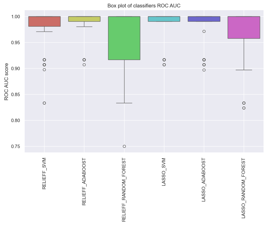
Fig. 4 The ROC AUC score for the predictive model with molecular data by using individual classifiers.
Example 3 - Construct the predictive model with molecular data by using ensemble learning
Ensemble configuration parameters
Required parameters
- X, variables (pd.DataFrame) X=X;
- y, target (pd.Series) y=y;
- features, list of feature sets (list) features=[relieff_features.features, lasso_features.features,];
- classifiers, list of classifiers (list) classifiers=['adaboost', 'random_forest', 'svm',];
- cv, cross-validation method (str) cv='stratified_k_fold';
- ensemble, list of ensemble methods (list) ensemble=['stacking',];
- repetitions, number of repetitions (int) repetitions=10;
Optional parameters
- classifier_params, classifiers hyperparameters (list of dicts) classifier_params=[{'adaboost': {'n_estimators': 100, 'learning_rate': 0.9,}}, {'random_forest': {'n_estimators': 100, 'criterion': 'gini', 'max_depth': None,}}, {'svm': {'C': 1, 'kernel': 'linear', 'gamma': 'auto'}},];
- cv_params, cross-validation method hyperparameters (dict) cv_params={'n_splits': 10};
- ensemble_params, ensemble hyperparameters (list of dicts) ensemble_params=[{'stacking': {'final_estimator': None,}},];
Stacking ensemble learning
ens_stacking = ens.Ensemble(
    X,
    y,
    features=[relieff_features.features, lasso_features.features,],
    classifiers=['adaboost', 'random_forest', 'svm',],
    classifier_params=[
        {'adaboost': {'n_estimators': 100, 'learning_rate': 0.9,}},
        {'random_forest': {'n_estimators': 100, 'criterion': 'gini', 'max_depth': None,}},
        {'svm': {'C': 1, 'kernel': 'linear', 'gamma': 'auto'}},
   ],
    cv='stratified_k_fold',
    cv_params={'n_splits': 10},
    ensemble=['stacking',],
    ensemble_params=[
        {'stacking': {'final_estimator': None,}},
    ],
    repetitions=10,
)
Get model metrics
ens_stacking.all_metrics()
["ACC: {'RELIEFF_STACKING': [0.993, 0.01], 'LASSO_STACKING': [0.994, 0.009]}",
 "Roc Auc: {'RELIEFF_STACKING': [0.981, 0.035], 'LASSO_STACKING': [0.984, 0.032]}",
 "F1 score: {'RELIEFF_STACKING': [0.996, 0.006], 'LASSO_STACKING': [0.997, 0.005]}",
 "MCC: {'RELIEFF_STACKING': [0.962, 0.054], 'LASSO_STACKING': [0.968, 0.051]}"]
Visualization of the model metrics
ens_stacking.plot_roc_auc()
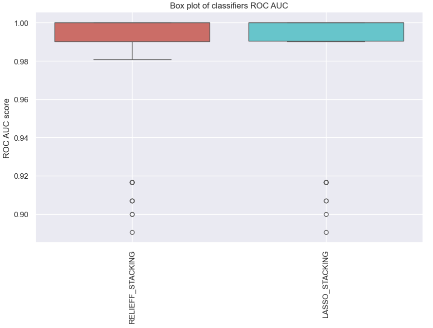
Fig. 5 The ROC AUC score for the predictive model with molecular data by using ensemble learning.
Voting ensemble learning
ens_voting = ens.Ensemble(
    X,
    y,
    features=[relieff_features.features, lasso_features.features,],
    classifiers=['adaboost', 'random_forest', 'svm',],
    classifier_params=[
        {'adaboost': {'n_estimators': 100, 'learning_rate': 0.9,}},
        {'random_forest': {'n_estimators': 100, 'criterion': 'gini', 'max_depth': None,}},
        {'svm': {'C': 1, 'kernel': 'linear', 'gamma': 'auto'}},
    ],
    cv='stratified_k_fold',
    cv_params={'n_splits': 10},
    ensemble=['voting',],
    ensemble_params=[
        {'voting': {'voting': 'soft'}},
    ],
    repetitions=10,
)

ens_voting.all_metrics()
Get model metrics
ens_voting.all_metrics()
["ACC: {'RELIEFF_VOTING': [0.991, 0.012], 'LASSO_VOTING': [0.995, 0.009]}",
 "Roc Auc: {'RELIEFF_VOTING': [0.98, 0.039], 'LASSO_VOTING': [0.989, 0.027]}",
 "F1 score: {'RELIEFF_VOTING': [0.995, 0.007], 'LASSO_VOTING': [0.997, 0.005]}",
 "MCC: {'RELIEFF_VOTING': [0.952, 0.061], 'LASSO_VOTING': [0.973, 0.047]}"]
Visualization of the model metrics
ens_voting.plot_roc_auc()
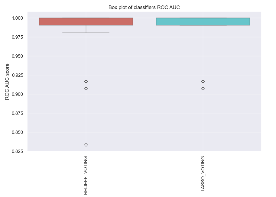
Fig. 6 The ROC AUC score for the predictive model with molecular data by using ensemble learning.
Bagging ensemble learning
ens_bagging = ens.Ensemble(
    X,
    y,
    features=[relieff_features.features, lasso_features.features,],
    classifiers=['adaboost', 'random_forest', 'svm',],
    classifier_params=[
        {'adaboost': {'n_estimators': 100, 'learning_rate': 0.9,}},
        {'random_forest': {'n_estimators': 100, 'criterion': 'gini', 'max_depth': None,}},
        {'svm': {'C': 1, 'kernel': 'linear', 'gamma': 'auto'}},
    ],
    cv='stratified_k_fold',
    cv_params={'n_splits': 10},
    ensemble=[
        'bagging',
    ],
    ensemble_params=[
        {'bagging': {
            'estimator_name': 'random_forest', 'n_estimators': 100, 'max_samples': 0.5, 'max_features': 0.5}},
    ],
    repetitions=10,
)

ens_bagging.all_metrics()
Get model metrics
ens_bagging.all_metrics()
["ACC: {'RELIEFF_BAGGING': [0.989, 0.013], 'LASSO_BAGGING': [0.987, 0.014]}",
 "Roc Auc: {'RELIEFF_BAGGING': [0.961, 0.052], 'LASSO_BAGGING': [0.962, 0.049]}",
 "F1 score: {'RELIEFF_BAGGING': [0.994, 0.007], 'LASSO_BAGGING': [0.993, 0.008]}",
 "MCC: {'RELIEFF_BAGGING': [0.94, 0.069], 'LASSO_BAGGING': [0.931, 0.072]}"]
Visualization of the model metrics
ens_bagging.plot_roc_auc()
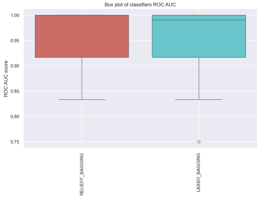
Fig. 7 The ROC AUC score for the predictive model with molecular data by using ensemble learning.
Release history Release notifications | RSS feed


Download files
Download the file for your platform. If you're not sure which to choose, learn more about installing packages.
Source Distribution
Built Distribution
Filter files by name, interpreter, ABI, and platform.
If you're not sure about the file name format, learn more about wheel file names.
Copy a direct link to the current filters
File details
Details for the file ensemble_binclass-1.0.12.tar.gz.
File metadata
- Download URL: ensemble_binclass-1.0.12.tar.gz
- Upload date:
- Size: 22.9 kB
- Tags: Source
- Uploaded using Trusted Publishing? No
- Uploaded via: twine/6.2.0 CPython/3.13.0
File hashes
| Algorithm | Hash digest | |
|---|---|---|
| SHA256 |
4bbacb7d2da29308765a7b47d95224878e0f42fbd29965a0a5e3d15db723e598
|
|
| MD5 |
ae8c2e8afe4aeef39e702afd07241e36
|
|
| BLAKE2b-256 |
6c043656a9fc761e060c70ea863f434086801ae56d3fe76544ffd5e3cd8c207c
|
File details
Details for the file ensemble_binclass-1.0.12-py3-none-any.whl.
File metadata
- Download URL: ensemble_binclass-1.0.12-py3-none-any.whl
- Upload date:
- Size: 20.9 kB
- Tags: Python 3
- Uploaded using Trusted Publishing? No
- Uploaded via: twine/6.2.0 CPython/3.13.0
File hashes
| Algorithm | Hash digest | |
|---|---|---|
| SHA256 |
5ceb47ced60481e38725320c54260db7c1a0fb1b8378bc4b1528a680e966319d
|
|
| MD5 |
47e22e11e8c9e7eca9e98585f120fb39
|
|
| BLAKE2b-256 |
3dc6516a00c55c00d1f4b5a6804dfebe45703b0b451597d8886046b9cdbb5138
|


