Tools for computing and visualizing ε-attracting basin


Project description
$\varepsilon$-Attracting Basin
Tools for computing and visualizing $\varepsilon$-attracting basin as introduced in Filtrations Indexed by Attracting Levels and their Applications. Y. Imoto and T. Yokoyama. arXiv:2506.18250.
Table of Contents
Overview
- Inputs are
- multiple sequence (time-series) data $Y=$ { $(y_1^{(i)}, y_2^{(i)}, \dots, y_{n_i}^{(i)}) \in \mathbb{R}^d\ | i=1,\dots,I$ }, where $i$ is a sequence index, $n_i$ is the number of sample (length) for the $i$ th sequence, and $d>0$ is the data dimension (assuming $y_{t+1}^{(i)} = F(y_{t}^{(i)})$ ),
- target cluster $A\subset Y$.
- Compute
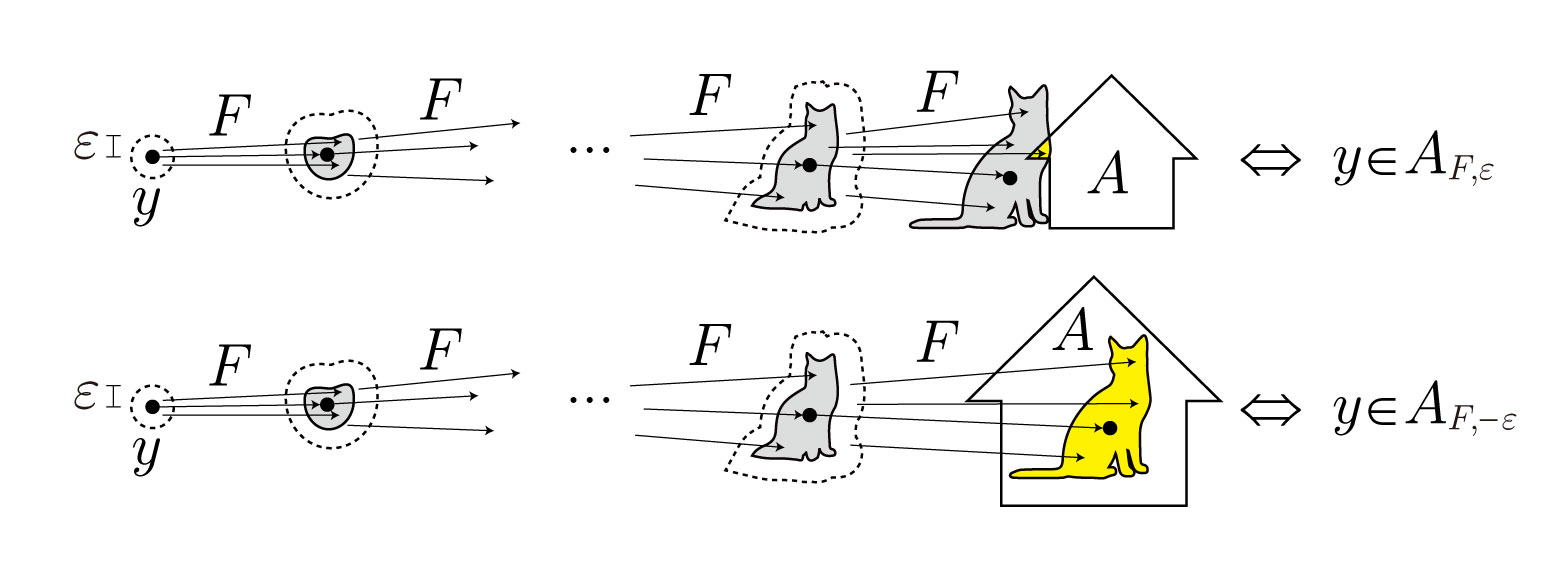
- $\varepsilon$-attracting basin $A_{F,\varepsilon}$, i.e., the set of states from which the system governed by $F$ can be driven into cluster $A$ by applying control of magnitude at most $\varepsilon>0$ at each time step.
- $-\varepsilon$-attracting basin $A_{F,-\varepsilon}$, i.e., the set of states in cluster $A$ from which the system cannot escape even if control of magnitude at most $\varepsilon>0$ is applied at each time step.
- $\varepsilon_{\Sigma}$-attracting basins $A_{F,\varepsilon_{\Sigma}}$ and $A_{F,-\varepsilon_{\Sigma}}$, i.e., the analogous sets when the total control energy over the entire sequence is at most $\varepsilon>0$.
For more theoretical background, see Filtrations Indexed by Attracting Levels and their Applications. Yusuke Imoto and Tomoo Yokoyama. arXiv:2506.18250.
Installation
You can install epsbasin either from PyPI or directly from the GitHub repository:
From PyPI:
pip install epsbasin
From GitHub:
git clone https://github.com/yusuke-imoto-lab/eps-attracting-basin.git
cd eps-attracting-basin
pip install -r requirements.txt
Usage
Put epsbasin.py in the same directory as the executable file and import it:
import epsbasin
Input Data Structure
The functions expect an anndata (annoted data matrix) object with the following structure:
-
.X
A numeric data matrix (observations/samples × features) used for computing pairwise costs if no precomputed cost matrix exists. -
.obs
A pandas DataFrame containing at least:'cluster': Categorical labels indicating cluster membership for each observation.'seq_id': Identifiers sequences (sequence index).
-
.uns(optional)'cost_matrix': Optional precomputed pairwise cost matrix (array of shape n_obs × n_obs). If absent, functions will compute it from.Xand store it here.
-
.obsm(optional)'plot_data': 2-dimensional data for 2D visualiztion plotting instead of.X.
Example of input data
For example, consider input data with two sequences, each having three time points $x^{(i)}_{j}~(i=1,2,~j=1,2,3)$ , where the final point of one sequence belongs to the “good” cluster and the final point of the other belongs to the “bad” cluster, as shown below:
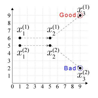
Then, the input anndata object adata should be constructed by
adara.X =
| 1 | 6 |
| 5 | 6 |
| 9 | 9 |
| 1 | 5 |
| 5 | 5 |
| 9 | 2 |
adata.obs =
| index | seq_id | cluster |
|---|---|---|
| 0 | 0 | other |
| 1 | 0 | other |
| 2 | 0 | good |
| 3 | 1 | other |
| 4 | 1 | other |
| 5 | 1 | bad |
import anndata
import panadas as pd

adata = anndata.AnnData(np.array([
    [1, 6],
    [5, 6],
    [9, 9],
    [1, 5],
    [5, 5],
    [9, 2]
]))
adata.obs = pd.DataFrame({
    "seq_id": [0, 0, 0, 1, 1, 1],
    "cluster": ["other", "other", "good", "other", "other", "bad"]
})
API Reference
$\varepsilon$-attracting basin
- Function:
eps_attracting_basin(adata, cluster_key="cluster", target_cluster_key="target_cluster", cost_matrix_key="cost_matrix", output_key="eps_attracting_basin", epsilon_delta=0.01) - Description: Compute the debut function
for the target cluster $A$ (indexed by
target_cluster_key) for input dataadata.X. If the cost matrix has not been precomputed (noadata.uns[cost_matrix_key]), the Euclidean distance matrix is calculated as the cost matrix.
$\varepsilon_\Sigma$-attracting basin
- Function:
eps_sum_attracting_basin(adata, cluster_key="cluster", target_cluster_key="target_cluster", cost_matrix_key="cost_matrix", output_key="eps_sum_attracting_basin", epsilon_delta=0.01) - Description: Compute the debut function
target_cluster_key) for input dataadata.X. If the cost matrix has not been precomputed (noadata.uns[cost_matrix_key]), the Euclidean distance matrix is calculated as the cost matrix.

Sublevel set visualization
- Function:
sublevel_set_visualization(adata, plot_key=None, eps_key="eps_attracting_basin", target_cluster_key="good", linewidth=0.5, color_name="_$\\varepsilon$", vmin=None, vmax=None, xlim=None, ylim=None, xlabel=None, ylabel=None, xticks=None, yticks=None, show_xticks=True, show_yticks=True, show_xlabel=True, show_ylabel=True, show_colorbar=True, show_colorbar_label=True, show_xticklabels=True, show_yticklabels=True, figsize=(10,8), levels=10, area_percentile=99.5, edge_percentile=99.5, save_fig=False, save_fig_dir=".", save_fig_name="sublevel_set_visualization") - Description: Visualize the $\varepsilon$- or $\varepsilon_\Sigma$-attracting basin (tha values on points are the debut function
or
) for the target cluster $A$ (indexed by
target_cluster_key) on a 2D Delaunay triangulation generated fromadata.X(oradata.obsm[plot_key]). Triangles with too large sides or areas can be removed by adjusting the parametersarea_percentileandedge_percentile.
Plot attracting basin
- Function:
plot_attracting_basin(adata, plot_key=None, eps_key="eps_attracting_basin", cluster_key="cluster", good_cluster_key="good", bad_cluster_key="bad", eps_threshold=0, background=None, figsize=(10,10), fontsize=14, pointsize=20, circ_scale=10, xlim=None, ylim=None, xlabel=None, ylabel=None, xticks=None, yticks=None, show_legend=True, show_label=True, show_ticks=True, show_title=True, title=None, label_clusters=["$G$","$B$"], label_basins=["$G_{F, \\varepsilon}$","$B_{F, \\varepsilon}$"], save_fig=False, save_fig_dir=".", save_fig_name="attracting_basin") - Description: Plot the $\varepsilon$- or $\varepsilon_\Sigma$-attracting basin of good and bad clusters (indexed by
good_cluster_keyancbad_cluster_key) by mapping 2D coordinates fromadata.Xoradata.obsm[plot_key].
For detailed usage, see espbasin.py.
Examples
- example_simple.ipynb: A simple exmaple of simulation data with one bifurcation in 2-dimensional space.
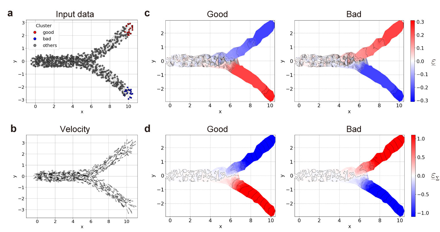
a, Input data with one bifurcation. b, Velocities of data (direction vectors of time increment $F(x)$ ). c, d, Distribution of debut functions $\underline{\varepsilon}$ (c) and $\underline{\varepsilon}_{\Sigma}$ (d) for clusters $G$ (reft) and $B$ (right).
- example_Dolphin.ipynb: An application exmaple of ensemble weather forecast data for tropical cyclone (typhoon), Dolphin, generated by the Meso-scale Ensemble Prediction System (MEPS), provided by the Japan Meteorological Agency (JSA).
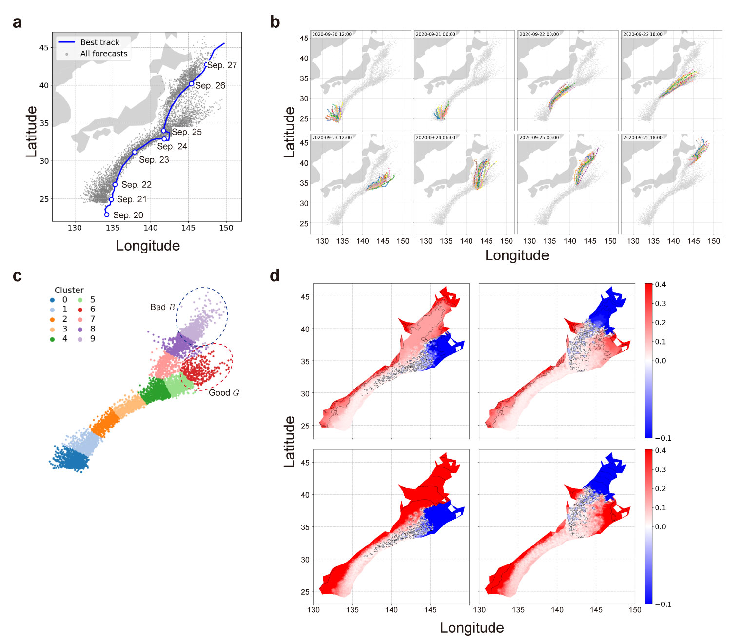
a, Best‐track trajectory (real orbit, blue line) overlaid with all forecast center positions (gray dots) of Dolphin. b, Selected ensemble forecast tracks at representative initial times. c, Clustering and assigning good and bad clusters. d, Distribution of debut functions $\underline{\varepsilon}$ (top) and $\underline{\varepsilon}_{\Sigma}$ (bottom) for clusters $G$ (reft) and $B$ (right).
- example_MEARI.ipynb: An application exmaple of ensemble weather forecast data for tropical cyclone (typhoon), MEARI, generated by the Meso-scale Ensemble Prediction System (MEPS), provided by the Japan Meteorological Agency (JSA).
Requirements
- Python ≥ 3.8
- numpy
- pandas
- scipy
- scikit-learn
- matplotlib
- anndata
Install all dependencies via:
pip install -r requirements.txt
License
MIT © 2025 Yusuke Imoto
Contact
- Yusuke Imoto
- Email: imoto.yusuke.4e@kyoto-u.ac.jp
- GitHub: yusuke-imoto-lab/eps-attracting-basin
Release history Release notifications | RSS feed


Download files
Download the file for your platform. If you're not sure which to choose, learn more about installing packages.
Source Distribution
Built Distribution
Filter files by name, interpreter, ABI, and platform.
If you're not sure about the file name format, learn more about wheel file names.
Copy a direct link to the current filters
File details
Details for the file epsbasin-0.2.0.tar.gz.
File metadata
- Download URL: epsbasin-0.2.0.tar.gz
- Upload date:
- Size: 13.5 kB
- Tags: Source
- Uploaded using Trusted Publishing? No
- Uploaded via: poetry/2.1.2 CPython/3.12.7 Linux/6.14.0-37-generic
File hashes
| Algorithm | Hash digest | |
|---|---|---|
| SHA256 |
cde70bef0fcb19f4a577b541ae2f0c837a913cdc24bf7176cfd6331c3ae2cdc4
|
|
| MD5 |
b0f42b0c6235dac433d72942c7be485f
|
|
| BLAKE2b-256 |
6d6d9187763bd6fd5801a422d1772764d9ec7c735b003a64630b7add8e388dd8
|
File details
Details for the file epsbasin-0.2.0-py3-none-any.whl.
File metadata
- Download URL: epsbasin-0.2.0-py3-none-any.whl
- Upload date:
- Size: 11.4 kB
- Tags: Python 3
- Uploaded using Trusted Publishing? No
- Uploaded via: poetry/2.1.2 CPython/3.12.7 Linux/6.14.0-37-generic
File hashes
| Algorithm | Hash digest | |
|---|---|---|
| SHA256 |
aed6999babe725a0e35b822d0779145ce3691cda9d879cad6305f9e0a515dfbe
|
|
| MD5 |
920a2c6cb3aeeb83817a2982680907bc
|
|
| BLAKE2b-256 |
4a7168b2074c7df23d298e786b52840a57e9aece7912dd3970ffe83758f5bee8
|


