







Read the ABSCAL.HIS file and visualize the results of the absolute calibration with liquid nitrogen of an RPG microwave radiometer
Table of Contents
Introduction
📖 Documentation: https://eval-ac.readthedocs.io (user guide, Python API, ABSCAL.HIS file format)
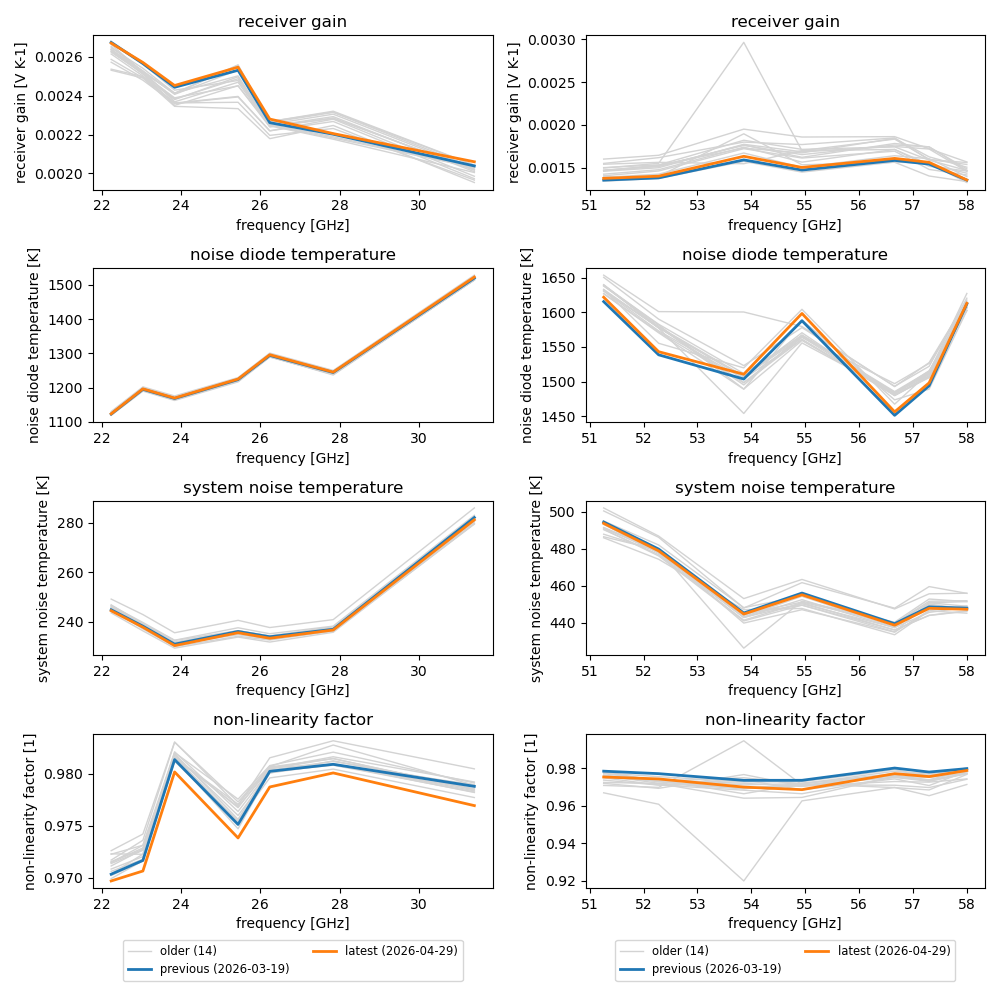
This repository was created to display the results of the absolute calibration with liquid nitrogen of the microwave radiometer HATPRO manufactured by Radiometer Physics GmbH. For this purpose, the binary file ABSCAL.HIS is read in and converted into an xarray. Then the receiver gain, the temperature of the noise diode, the temperature of the system noise and the non-linearity factor are displayed in comparison to the previous and other prior calibrations.
Getting Started
Installation
eval_ac requires Python 3.9 or newer. The dependencies (numpy, xarray, matplotlib, netCDF4) are installed automatically.
-
Clone the repo
git clone https://github.com/WillyWallace/eval_ac.git
cd eval_ac
-
Install the package
pip install .
For development (editable install with test and lint tools):
pip install -e ".[dev]"
Usage
Command line
eval-ac path/to/ABSCAL.HIS --netcdf abscal.nc
This writes the NetCDF file, the history plot results_ln2_cal.png, the drift plot results_ln2_drift.png and prints a short quality report of the latest calibration:
read 16 calibration entries from path/to/ABSCAL.HIS
16 of them are calibrations with liquid nitrogen
receiver 1: latest calibration 2026-04-29 (159 days ago)
receiver 2: latest calibration 2026-04-29 (159 days ago)
drift: all channels of the latest calibration are within the thresholds
Lines starting with warning: point to something that should be checked, see Quality checks.
| Option | Description |
|---|---|
input |
path of the ABSCAL.HIS file (required) |
-n, --netcdf FILE |
write the converted data (all calibration types) to a NetCDF file |
-p, --plot FILE |
file name of the history plot (default: results_ln2_cal.png) |
-d, --drift-plot FILE |
file name of the drift plot (default: results_ln2_drift.png) |
--no-plot |
do not create any plot |
--show |
additionally show the plots in a window |
--all-cal-types |
use all calibrations instead of only those with liquid nitrogen |
--n-reference N |
number of calibrations before the latest one forming the drift reference (default: 5) |
-t, --threshold VAR=PERCENT |
drift threshold, e.g. -t gain=8 -t temp_sys=2; variables: gain, temp_noise, temp_sys, alpha |
--max-age DAYS |
warn if the latest calibration of a receiver is older (default: 183 days) |
--fail-on-warning |
exit with code 2 if the report contains a warning (e.g. for cron jobs) |
--version |
print the version |
python -m eval_ac ... works as well. Try it with the example file:
eval-ac example_data/ABSCAL.HIS
History plot
The plot shows the receiver gain, the noise diode temperature, the system noise temperature and the non-linearity factor of both receivers. The latest and the previous calibration of each receiver are highlighted with their dates, all older calibrations are drawn in grey. Channels that were not calibrated (calibration_flag = 0) are marked with a red cross. By default, only calibrations with liquid nitrogen are used (cal_type = 1); if only one receiver of an entry was calibrated with liquid nitrogen, only this receiver is used.
Drift plot
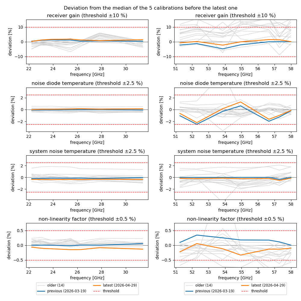
For each receiver, the latest calibration is compared with the median of the 5 calibrations before it (deviation in percent). Channels that were not calibrated are excluded. The dashed red lines are the thresholds, channels of the latest calibration exceeding them are circled and listed in the report. The grey lines show how far the older calibrations deviate from the same reference.
The y-axis is scaled to the thresholds and to the latest and previous calibration. Large outliers of older calibrations are therefore cut off at the edge of the panel; they are still visible in the history plot.
Quality checks
The report checks the latest calibration of each receiver (only calibrations with liquid nitrogen, unless --all-cal-types is given):
| Check | Warning if | Background |
|---|---|---|
| Age | the latest calibration is older than --max-age days (default 183) |
RPG recommends an absolute calibration every 5 to 6 months and after transport (manual, section 3.1.3). The age is computed from the calibration time of each receiver. |
| Flag | a channel has calibration_flag = 0 |
The channel was not calibrated (manual, appendix A20). |
| Non-linearity factor | α is outside 0.9 ≤ α < 1 | Valid range of the detector model (manual, section 3.1.3.1, equation 1). Channels with flag 0 are not checked. |
| Drift | the deviation from the reference exceeds the threshold | See Drift plot and Interpreting the results. |
With --fail-on-warning, eval-ac exits with code 2 if any check gives a warning, e.g. to send an e-mail from a cron job:
eval-ac /data/ABSCAL.HIS --no-plot --fail-on-warning || echo "check calibration" | mail -s "HATPRO" me@example.org
Interpreting the results
The report and the drift plot point to calibrations that deserve a closer look; they do not decide whether a calibration is good or bad. That decision needs the knowledge of the instrument and of the calibration conditions. The background below is taken from the RPG manual Principle of Operation & Software (standard radiometers), RPG-MWR-STD-SW (cited as "manual, section …").
What the absolute calibration determines
During the absolute calibration the radiometer looks at the internal ambient target and at the external liquid nitrogen cooled target, each with and without additional noise from the noise diode. From these four measurements it determines four parameters per channel (manual, section 3.1.3.1):
| Variable | Meaning | Use between two absolute calibrations |
|---|---|---|
gain (G) |
receiver gain [V/K] | Very sensitive to small changes of the physical temperature of the receiver; it is recalibrated regularly with the ambient target (gain calibration, manual, section 3.3). |
temp_sys (Tsys) |
system noise temperature [K] | Recalibrated together with G using the noise diode and the ambient target (manual, section 3.1.3.1). Changes of the temperature of the receiver optics (e.g. the feedhorn) change Tsys (manual, section 3.1.3.2). |
temp_noise (Tn) |
equivalent temperature of the noise diode [K] | Used as secondary standard for all automatic calibrations until the next absolute calibration; it is assumed to be stable (manual, section 3.1.3.1). In transparent channels it can also be recalibrated by sky tipping (manual, section 4.9.1). |
alpha (α) |
non-linearity factor of the detector, U = G·Pα with 0.9 ≤ α < 1 | Assumed to be constant until the next absolute calibration (manual, section 3.1.3.1). |
Consequences for the evaluation
- Changes of Tn and α are the most relevant: until the next absolute calibration, every automatic calibration builds on them. A real change of Tn that is not captured by a new absolute calibration enters the measured brightness temperatures.
- Differences of the gain between absolute calibrations are expected, because the gain follows the receiver temperature and is recalibrated during operation anyway. Its default threshold is therefore larger. In the example data the gain varies much more than the other variables (standard deviation 1–3 % in the K-band and 5–18 % in the V-band, compared with below 2 % for Tn and Tsys).
- ABSCAL.HIS also contains successful sky tipping calibrations (manual, section 4.6). They use a different method and are only possible in transparent channels, so eval_ac compares only calibrations with liquid nitrogen by default.
Why the median of the previous calibrations?
A single failed calibration in the reference would shift a mean, but hardly the median. The previous calibration is part of the reference, so its deviation is usually small.
Typical patterns
These are rules of thumb, not statements of the manual:
| Pattern in the drift plot | Possible meaning |
|---|---|
| Latest within the thresholds, similar to the grey lines | Calibration consistent with the history. |
| Single channels of the latest calibration out of the thresholds, previous calibration normal | Possibly a problem during this calibration, e.g. with the cold target (filling, condensation; the manual asks to let the target dry before the V-band part, section 4.8). Check the calibration conditions and consider repeating the calibration. |
| All channels of a receiver shifted in the same direction | Rather a change of the receiver or of its noise diode than a single failed calibration, e.g. after maintenance or transport. |
| Latest and previous calibration deviate in the same way | The change is confirmed by two calibrations and is probably real; the reference (the 5 calibrations before) still describes the old state. |
| Channels marked as "not calibrated" (flag 0) | These channels were not calibrated in this entry (manual, appendix A20); they are not evaluated. |
What to do with a suspicious calibration
- Check that the absolute calibration was done after a warm-up of at least 30 minutes; it is recommended every 5 to 6 months and after transport (manual, section 3.1.3).
- Repeat the calibration if the conditions were doubtful.
- A bad calibration can be removed in the RPG host software: in the Absolute Calibration History menu, Delete Last Entries removes all entries after the marked one, and Generate a new calibration file creates an ABSCAL.CLB from selected calibrations of receiver 1 and 2 (manual, section 4.6).
Adapting the thresholds
The default thresholds are derived from a single HATPRO (2018–2026, 16 calibrations). Instruments, channels and sites differ, so:
- run
eval-acon the full history of your instrument, - look at the spread of the grey lines in the drift plot,
- set thresholds slightly above the usual spread, e.g.
-t gain=6 -t temp_noise=1.5.
Limitations
- With fewer than 5 earlier calibrations, the reference consists of fewer values (see
n_reference_usedin the result ofcalibration_drift()); with none, no drift can be computed. - The drift is relative to the previous calibrations. A slow drift over many calibrations shifts the reference as well and is better seen in the history plot.
Python
from eval_ac.convert_abscal_his import read_abscal_his, write_netcdf
from eval_ac.analysis import select_cal_type, calibration_drift, drift_exceedances
from eval_ac.plotting import plot_calibration_history, plot_drift

ds = read_abscal_his("ABSCAL.HIS")   # xarray.Dataset, all calibration types
write_netcdf(ds, "abscal.nc")

ln2 = select_cal_type(ds)            # only calibrations with liquid nitrogen
fig = plot_calibration_history(ln2, variables=["gain", "temp_sys"])
fig.savefig("gain_tsys.png")

drift = calibration_drift(ln2, n_reference=5)
for row in drift_exceedances(drift, thresholds={"gain": 8}):
    print(row)
plot_drift(drift, thresholds={"gain": 8}).savefig("drift.png")
The dataset has the dimensions n_samples (calibration entries, oldest first) and freq (channels). The coordinate time holds the date of each calibration, the coordinate receiver (1 or 2) assigns each channel to its receiver.
Running the tests
pip install -e ".[test]"
pytest
Roadmap
- add meaningful docstrings
- make documentation with Sphinx (
docs/) - host the documentation on readthedocs
- enable pip install ...
- publish on PyPI
- Released version 1
- Add Tests
See the open issues for a full list of proposed features (and known issues) and CHANGELOG.md for the changes of each version.
License
Distributed under the MIT License. See LICENSE for more information.
Contact
Acknowledgments
Special thanks for templates and help during implementation.
1 maintainer

Metadata
1 maintainer
Release files for eval-ac 0.3.1
For a detailed explanation of source distributions (sdists) and built distributions (wheels), please see the package formats documentation.
Source distribution (sdist)
| File | Size | Uploaded | |
|---|---|---|---|
| eval_ac-0.3.1.tar.gz | 44.9 kB | Details |
Built distribution (wheel)
| File | Interpreter | ABI | Platform | Reset |
|---|---|---|---|---|
| eval_ac-0.3.1-py3-none-any.whl | Python 3 | none | any | Details |
Total release size: 69.5 kB
Release files / eval_ac-0.3.1.tar.gz
| Download URL | eval_ac-0.3.1.tar.gz |
|---|---|
| Size | 44.9 kB |
| Tags | Source |
|
SHA-256 checksum How to use checksums |
d0895a200c80d20087c8dfb6524df6f99498dcfa465645358386d7a848fa8a16
|
|
BLAKE2b-256 checksum How to use checksums |
98f33caca33b55330bf0cf6cb280ecd7eeb3814bdde57f405c8e878ef92787fb
|
| Upload date | |
|
Uploaded using Trusted Publishing? What is trusted publishing? |
Yes |
| Uploaded via |
twine/7.0.0 CPython/3.13.14
|
Provenance
Provenance describes where a file came from. On PyPI, provenance is shared via attestations, which provide a verifiable record of the build or publishing details. View details, limitations and caveats.


PyPI Publish Attestation
PyPI verified that this artifact, at this checksum, originated from the publisher listed below.
Signed by GitHub Actions, verified by PyPI on Oct 6, 2026.
Transparency logRelease files / eval_ac-0.3.1-py3-none-any.whl
| Download URL | eval_ac-0.3.1-py3-none-any.whl |
|---|---|
| Size | 24.5 kB |
| Tags | Python 3 |
|
SHA-256 checksum How to use checksums |
55d0dd006fba776214d12516bee4ea28656643a5bc8c77c10d86e8a4b5228518
|
|
BLAKE2b-256 checksum How to use checksums |
64b0673fe36cdcefe79784f81a5f2082e163faa861130b5f86cce9705008be98
|
| Upload date | |
|
Uploaded using Trusted Publishing? What is trusted publishing? |
Yes |
| Uploaded via |
twine/7.0.0 CPython/3.13.14
|
Provenance
Provenance describes where a file came from. On PyPI, provenance is shared via attestations, which provide a verifiable record of the build or publishing details. View details, limitations and caveats.
PyPI Publish Attestation
PyPI verified that this artifact, at this checksum, originated from the publisher listed below.
Signed by GitHub Actions, verified by PyPI on Oct 6, 2026.
Transparency log












