
py-excel-solver 
A wrapper that uses Scipy's linprog() function to emulate the UI of Excel's Solver. It's supposed to be extremely easy to use. If you've set up a simple optimization problem in Excel, just copy and paste the values into the function below and get the same output.
Source code
Install
pip install excel_solver
How to use
- Download
solver.py(click 'raw' view, then right click, Save As) import solver, then follow the format of the implementations below- Optional: download
example-code.pyand execute it from same folder as solver.py to test it out.
Params for solver.solve():
- problem_type: Required. Specify "max" or "min"
- objective_function: Required. List of coefficients.
- constraints_left: Required. Constraint matrix, where columns correspond to objective function coefficients. Can be 2d list or np arr.
- constraints_right: Required. These are constraint vectors used to make the comparison.
- constraints_signs: Required. A list of signs corresponding to your constraints. Allowed:
>=, <=, = - make_unconstrained_non_negative: (optional) Just like the button in Excel. Setting this to False is the same as setting minimum_for_all to None.
- minimum_for_all: (optional) Set the lower limit for all decision variables.
- maximum_for_all: (optional) Set the upper limit for all decision variables.
- bounds: (optional) default None. Use this to specify custom bounds for each var individually. Pass an array of tuples [(), (), etc.].
- method: (optional) default simplex. You can pass any of the ones listed in Scipy documentation.
- display_result: (optional) default True
Rules:
- All matrix constraints must be able to be stated with a SUMPRODUCT() in Excel. Instead of passing the sumproduct cell as a constraint like you would in Excel, here you need to pass the constraint matrix itself (see
constraints_leftparam below), and the function will take care of the math.
Why use this?
- It's easy. Very easy. You can simply copy paste from excel into the function. You even get to use the "Make Unconstrained Variables Non-Negative" button, like you would in Excel.
Extra features you don't get in Excel Solver
- With a single-integer assignment, you can set the
minimum_for_alland/ormaximum_for_allconstraints to set an upper and/or lower bound for all the decision variables at once. - You don't have to calculate objective function or matrix sumproduct constraints yourself.
- Objective function is set up and displayed for you in the output. Ex:
MINIMIZE: z = 16a - 20.5b + 14c. - Choose from a variety of solve methods not offered in Excel.
Why not just use scipy.optimize.linprog()?
- Scipy's
linprog()is very hard to use if you're coming from Excel. It does NOT let you pick between maximize and minimize like you would in Excel, and it does not let you specify inequality signs (>= <=) for constraints. And, if you want to assert equalities as constraints, you have to pass them as a completely separate matrix/vector pair in the function. As a result, using scipy linprog() requires that you manipulate many of your values ahead of time in a way that makes your code impossible to read and interpret.
Example 1
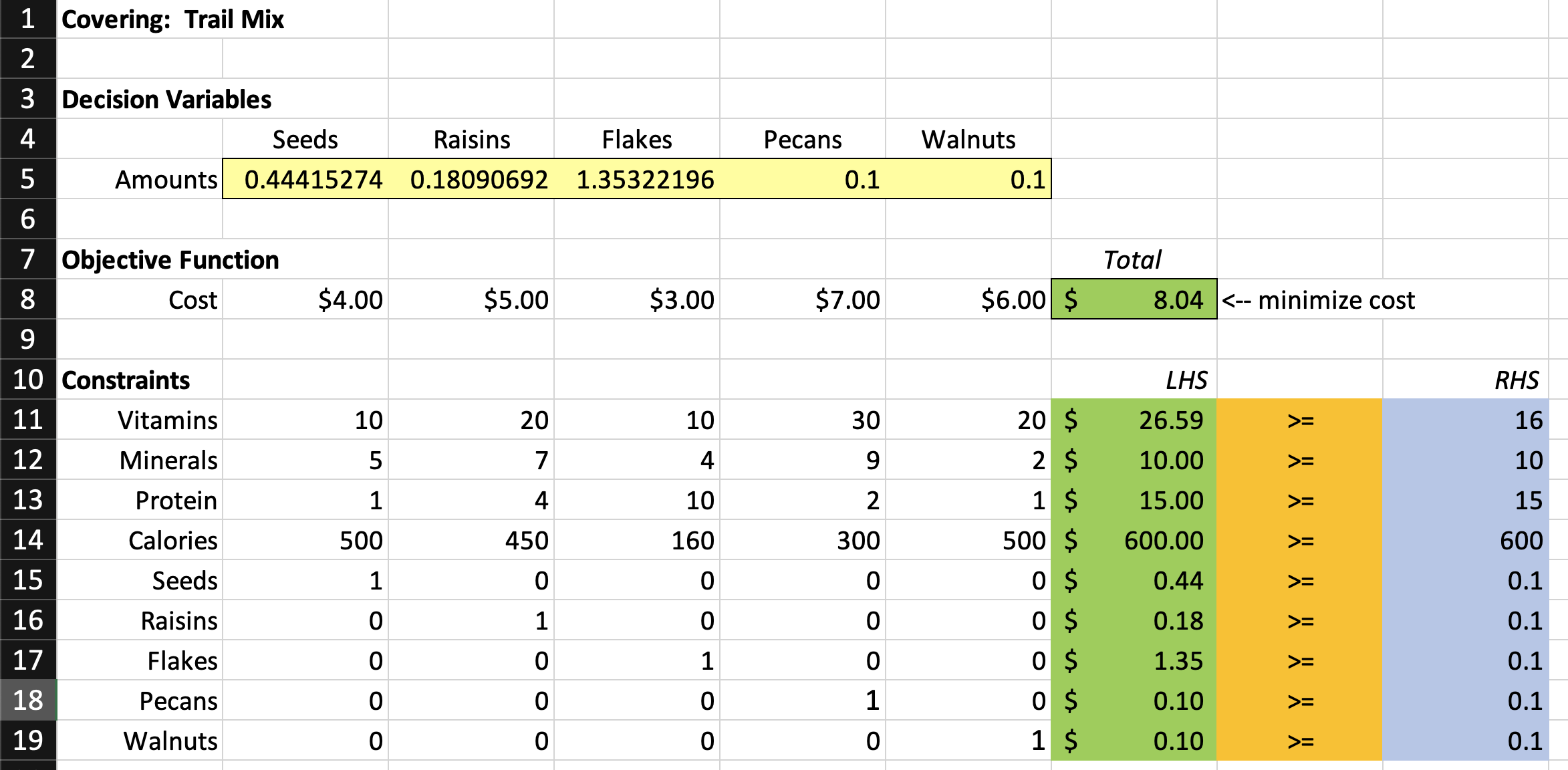
Solved in Excel:
Solved in Python:
Code:
import solver
solver.solve(
    problem_type = "min",
    objective_function = [
        4, 5, 3, 7, 6
    ],
    constraints_left = [
        [10,  20,  10,  30,  20],
        [5,   7,   4,   9,   2],
        [1,   4,   10,  2,   1],
        [500, 450, 160, 300, 500],
    ],
    constraints_right = [
        16,
        10,
        15,
        600,
    ],
    constraints_signs = [
        ">=",
        ">=",
        ">=",
        ">=",
    ],
    minimum_for_all=0.1, # replaces lines 15-19 in the excel image above
)
Output:
------------------------------------------------------
MINIMIZE: z = 4a + 5b + 3c + 7d + 6e
------------------------------------------------------
OPTIMAL VALUE:  8.04
------------------------------------------------------
QUANTITIES:
a:  0.44415
b:  0.18091
c:  1.35322
d:  0.1
e:  0.1
------------------------------------------------------
Optimization terminated successfully. (HiGHS Status 7: Optimal)
Example 2
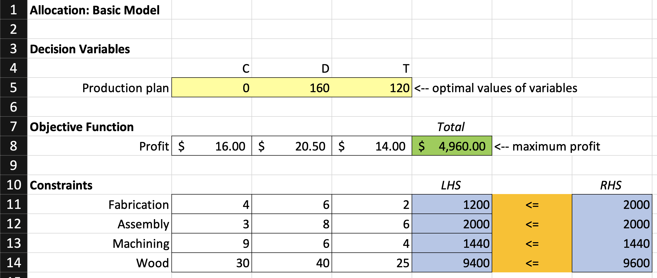
Solved in Excel:
Solved in Python:
Code
import solver
solver.solve(
    problem_type = "max",
    objective_function = [
        16, 20.5, 14
    ],
    constraints_left = [
        [4,  6,  2],
        [3,  8,  6],
        [9,  6,  4],
        [30, 40, 25],
    ],
    constraints_right = [
        2000,
        2000,
        1440,
        9600,
    ],
    constraints_signs = [
        "<=",
        "<=",
        "<=",
        "<=",
    ],
)
Output
------------------------------------------------------
MAXIMIZE: z = 16a + 20.5b + 14c
------------------------------------------------------
OPTIMAL VALUE:  4960
------------------------------------------------------
QUANTITIES:
a:  0
b:  160
c:  120
------------------------------------------------------
Optimization terminated successfully. (HiGHS Status 7: Optimal)
Now, let's try switching the 2nd constraint in the previous problem from '<= 2000' to '= 1984'. If you were using Scipy, this wouldn't be possible without making two new separate arrays to store this constraint.
NOTE: This is NOT necessary, but I've re-ordered the constraints so the equality is on the bottom. You can have them in any order you like.
Code
import solver
solver.solve(
    problem_type = "max",
    objective_function = [
        16, 20.5, 14
    ],
    constraints_left = [
        [4,  6,  2],
        [9,  6,  4],
        [30, 40, 25],
        [3,  8,  6],
    ],
    constraints_right = [
        2000,
        1440,
        9600,
        1984,
    ],
    constraints_signs = [
        "<=",
        "<=",
        "<=",
        "=",
    ],
)
Output
------------------------------------------------------
MAXIMIZE: z = 16a + 20.5b + 14c
------------------------------------------------------
OPTIMAL VALUE:  4952
------------------------------------------------------
QUANTITIES:
a:  0
b:  176
c:  96
------------------------------------------------------
Optimization terminated successfully. (HiGHS Status 7: Optimal)
1 maintainer

Metadata
1 maintainer
Release files for excel-solver 0.0.0
For a detailed explanation of source distributions (sdists) and built distributions (wheels), please see the package formats documentation.
Source distribution (sdist)
| File | Size | Uploaded | |
|---|---|---|---|
| excel_solver-0.0.0.tar.gz | 216.7 kB | Details |
Built distribution (wheel)
| File | Interpreter | ABI | Platform | Reset |
|---|---|---|---|---|
| excel_solver-0.0.0-py3-none-any.whl | Python 3 | none | any | Details |
Total release size: 224.0 kB
Release files / excel_solver-0.0.0.tar.gz
| Download URL | excel_solver-0.0.0.tar.gz |
|---|---|
| Size | 216.7 kB |
| Tags | Source |
|
SHA-256 checksum How to use checksums |
8dc01aaffefea88ca57a934e8dc4b58effc6a829f6fac19f9a843e82420354f8
|
|
BLAKE2b-256 checksum How to use checksums |
e8c751381a0e065c12afdfb6f6329371462eef2bc05b55ddd8831186d216345c
|
| Upload date | |
|
Uploaded using Trusted Publishing? What is trusted publishing? |
No |
| Uploaded via |
twine/4.0.1 CPython/3.11.0
|
Release files / excel_solver-0.0.0-py3-none-any.whl
| Download URL | excel_solver-0.0.0-py3-none-any.whl |
|---|---|
| Size | 7.3 kB |
| Tags | Python 3 |
|
SHA-256 checksum How to use checksums |
4da282dc56511ab9d136146ee2627c115c9961b234eb53fc90ad291f0eaab07d
|
|
BLAKE2b-256 checksum How to use checksums |
2150775491fa59bba32895fee4f5616a0c50598bffe87ee8872d49ae2f0861bb
|
| Upload date | |
|
Uploaded using Trusted Publishing? What is trusted publishing? |
No |
| Uploaded via |
twine/4.0.1 CPython/3.11.0
|













