
GUI program for aperture photometry of known exoplanet transits. Image reduction, light curve construction, analysis and transit modeling

Project description
ExoPhotoCurve -- EPC --
📖 Author: Daniele Gasparri
📅 Latest Release: June 2026


ExoPhotoCurve is a GUI program designed to create, inspect, correct, analyze and model photometric light curves of known exoplanet transits. It is particularly suited for follow-up observations and fast modeling, using the embedded NASA and ExoClock catalogs.
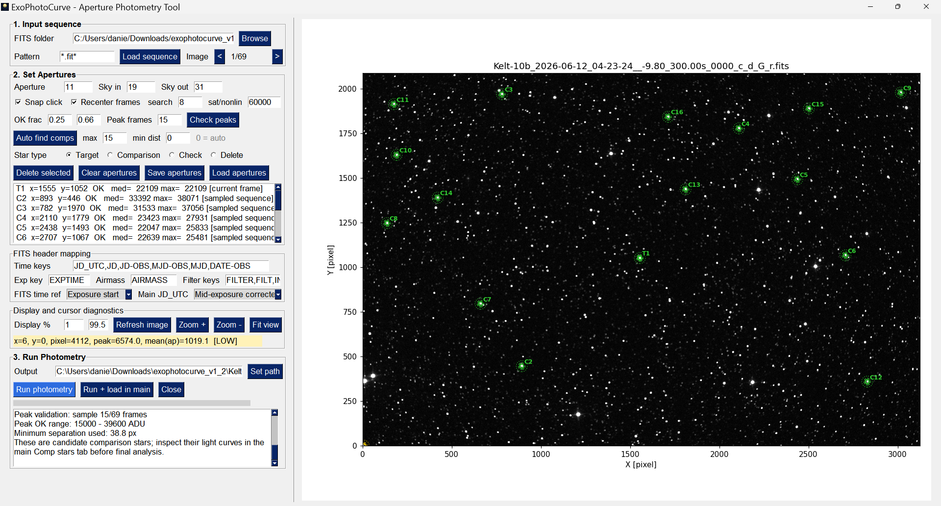
Aperture photometry module
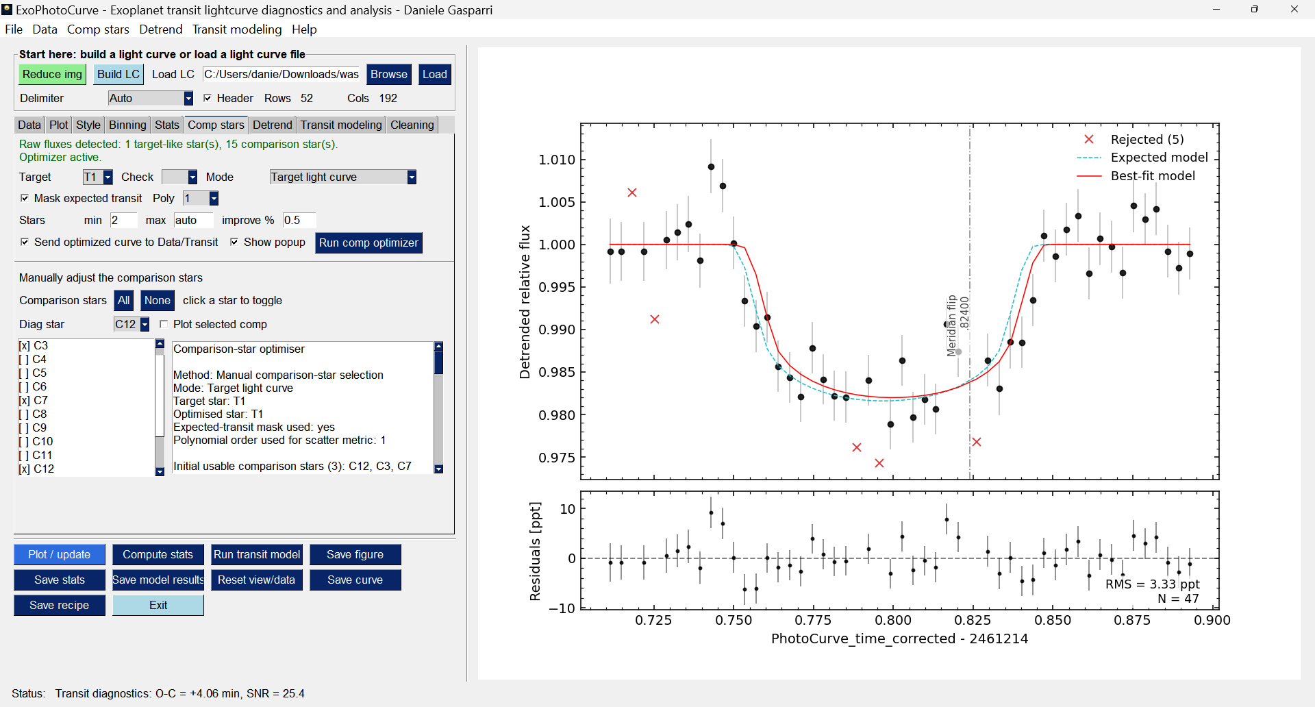
Light curve analysis module
Features
- Full reduction of raw image sequence using rigorous approach to preserve and maximize the photometric information:
- Calibration of raw FITS images with bias, dark and flat frames
- Automatic alignment handling translation, rotation and meridian flip
- Monochrome and color data handling. For color data, user selected channel extraction is performed without applying the debayer process
- Differential aperture photometry from calibrated and aligned FITS images:
- Automatic fits sequence recognition
- Interactive aperture adjustment and positioning
- Automatic visual feedback to let the user know if a target or comparison star are within the optimal linear range
- Automatic centroid recentering on all the images of the loaded sequence
- Saving apertures to be loaded any time
- Photometry file generated compatible with AstroImageJ and automatically passed to the analysis panel
- Light curve fine-tuning, analysis, and transit modeling:
- Interactive plot window updated in real time
- Automatic or manual clipping of outliers
- Automatic or manual selection of the comparison stars to optimize the signal-to-noise of the transit
- Detrending methods: airmass, JD_UTC, FWHM, and meridian flip correction
- Transit modeling using the physical data of the considered extrasolar planet and comparison with the expected model, using the embedded NASA and ExoClock extrasolar planet databases.
- Saving plot, statistics, diagnostics and the full recipe in order to grant reproducibility.
System Requirements
- Python 3.10+
- Screen resolution of at least 1600x900 px. Optimal resolution: 1920X1080
- The following dependencies will be automatically installed: numpy, pandas, matplotlib, scipy, astropy, astropy-iers-data, batman-package
- A 64 bit standalone Windows installer (no Python required) is also available in the GitHub official release page (https://github.com/danielegasparri/ExoPhotoCurve/releases/download/v1.1.0/ExoPhotoCurve-1.1.0-Windows-x64-Setup.exe).
Installation
You can install ExoPhotoCurve using pip:
pip3 install exophotocurve
or using the Windows installer, for 64 bit Windows 10+ systems.
Quick Start
Run ExoPhotoCurve using:
exophotocurve
You can download an example reduced sequence of the planet Kelt-10b transit in the official GitHub ExoPhotoCurve release page (https://github.com/danielegasparri/ExoPhotoCurve/releases/download/v1.0.0/Kelt-10b_2026-06-12_reduced.zip), and start playing with the program.
Quick start with example dataset
Build the raw light curve:
- Unzip the reduced sequence
- Open ExoPhotoCurve and click on "Build LC"
- Browse the sequence folder, confirm and click to "Load sequence"
- Leave the apertures with their default size, move the mouse on the plot to see the aperture annulus
- Zoom in the center with mouse wheel or scroll touch of the touchpad and place the aperture to the bright star in the center (the target). In the sequence folder you will find a chart to help you identify the target (called T1)
- Click to "Auto find comps": ExoPhotoCurve will find the best 15 comparison stars for you. You can verify they are good because the apertures will be all green, otherwise they would have been yellow (stars too faint) or red (stars near saturation or saturated)
- Go to "3. Run Photometry" and click to "Set path" to set the path and the name of the raw light curve. I suggest to put the name of the planet, so ExoPhotoCurve will recognize it automatically during the analysis. Something like that: "Kelt-10b_lightcurve"
- Click "Run + load in main": ExoPhotoCurve will perform the differential photometry, close the window and automatically load the light curve file in the main panel
Fine-tuning and analyze the raw light curve:
- In the main panel, now click "Plot / Update" to see the first, raw light curve. Congratulations!
- Now we need to check the comparison stars in the "Comp stars" tab. You can take a look at any single comparison, or try to deselect some of them to see how the transit light curve will adapt. If you trust me, deselect the C4 and C16 stars and leave the others selected: this is, for me, the best combination of comparison stars that gives you a sharp and symmetric light curve.
- We notice in the plot a point quite off the main trend, just on the right, out of the transit event. We can go to the "Cleaning" tab, activate the "Click-edit plot" option and click on this point to turn it off from the light curve.
- Now it's time for the first fit. Go to the "Transit modeling" tab, make sure the planet is recognized in the "Planet" section, otherwise select it manually, and just click the button "Run transit model" below. This is your first fit, a solid base to improve the results.
- During the acquisition of this sequence, the mount of the telescope had to perform the meridian flip. Usually this produces a little jump in the light curve. You cannot see it, but it's there and it's the main reason why the fit do not overlap with the expected model. Let's go to the "Detrend" tab and activate the "Meridian flip" option. In "time frac" you should insert the JD fraction where the meridian flip occurred. If you trust me, put here: .770. Click on the "Plot / update" button to show the vertical line of the meridian flip time.
- Activate the "Consider fit model" and in the "Model-aware mod" select "Iterate to convergence". ExoPhotoCurve will use this rough fit as a base to correct iteratively for the subtle meridian flip jump. Click on "Run detrending" and look at the result. Now the fit improved a lot and it is very similar to the expected model!
- The final light curve is ready. If you want to play more, you may go to the "Cleaning" section again and apply an automatic sigma clipping to delete the outlier points. Set the "Sigma" to 2.5 (very aggressive, just to try) and click on "Apply sigma clipping". Remember to do the fit again if any point is deleted by clicking "Run transit model". The final result should appear very similar (hopefully the same) to this:
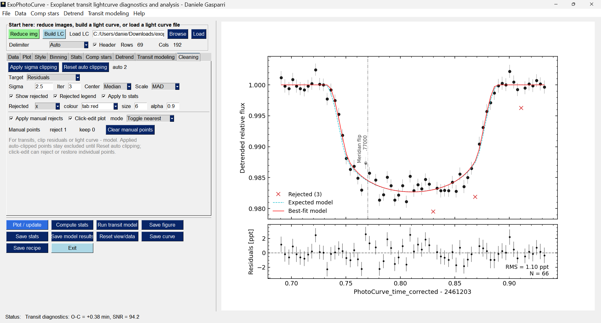
If not, try to start from fresh by clicking the button "Reset view/data" and try again.
Now that you are satisfied you can save the plot, but especially you should save this final light curve with the button "Save curve". ExoPhotoCurve will save two files in ASCII format, one containing the detailed light curve with detrend and model, and the second with only the relevant columns (time, flux, errors) ready to be uploaded to the ExoClock or ETD platforms.
License
ExoPhotoCurve is licensed under the non-commercial License. See the LICENSE file for details.
Contact & Contributions
Found a bug? Want to suggest a feature?
Drop me an email!
Contact: Daniele Gasparri – daniele.gasparri@gmail.com
Take a look also at my website, if you are interested in astronomy: https://www.danielegasparri.com/
Release history Release notifications | RSS feed

Download files
Download the file for your platform. If you're not sure which to choose, learn more about installing packages.
Source Distribution
Built Distribution
Filter files by name, interpreter, ABI, and platform.
If you're not sure about the file name format, learn more about wheel file names.
Copy a direct link to the current filters
File details
Details for the file exophotocurve-1.1.0.tar.gz.
File metadata
- Download URL: exophotocurve-1.1.0.tar.gz
- Upload date:
- Size: 2.5 MB
- Tags: Source
- Uploaded using Trusted Publishing? No
- Uploaded via: twine/6.2.0 CPython/3.13.14
File hashes
| Algorithm | Hash digest | |
|---|---|---|
| SHA256 |
18602a8bc11af6154bd65024815a1c616cb855a508d913f1d901f20b49d5dc7c
|
|
| MD5 |
7d328d1180b51abb1969256f57b23daa
|
|
| BLAKE2b-256 |
5b29b8b35a61ce1f1f59f39d29f15b1a10813297c76362a2632346434fc45e44
|
File details
Details for the file exophotocurve-1.1.0-py3-none-any.whl.
File metadata
- Download URL: exophotocurve-1.1.0-py3-none-any.whl
- Upload date:
- Size: 2.5 MB
- Tags: Python 3
- Uploaded using Trusted Publishing? No
- Uploaded via: twine/6.2.0 CPython/3.13.14
File hashes
| Algorithm | Hash digest | |
|---|---|---|
| SHA256 |
e11cb109c015200ed62af4b2087dd6af9a4b25c996249998d4ac2af51d4dab9f
|
|
| MD5 |
98947b44edb3e60e0839d19be976a05a
|
|
| BLAKE2b-256 |
679c94b44a57927ec4f793d9cc7d672c6e01ea7eb436220c01e490334ac63716
|






