
Overview of EYKTHYR
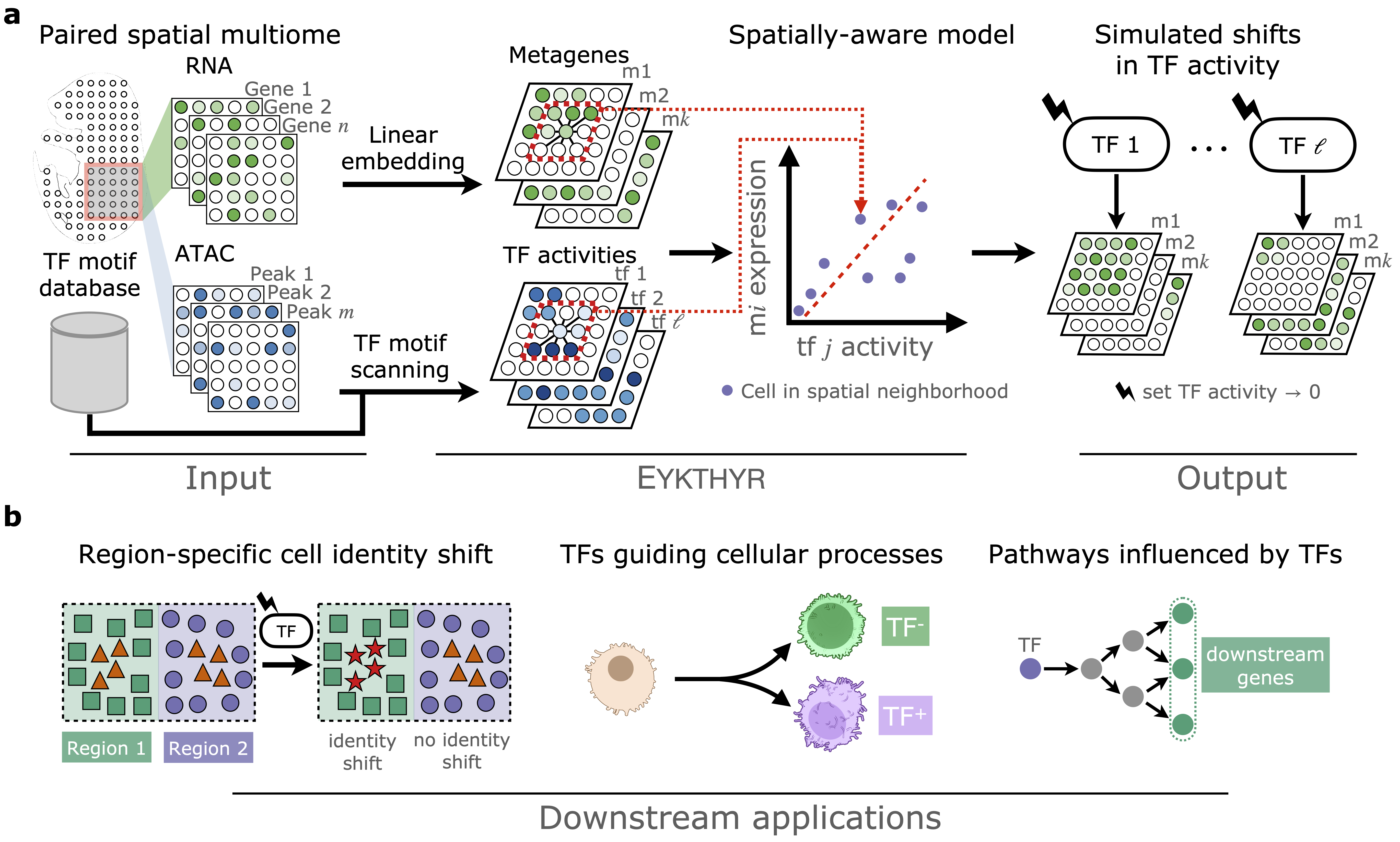
EYKTHYR is the first method developed to infer region-specific TF influences on spatial gene programs (or metagenes) using spatial multiome data. EYKTHYR addresses high technical dropout by introducing a novel combination of linear embeddings for gene expression and chromatin accessibility, denoising the data while maintaining interpretability, as shifts in metagene embeddings map directly back to input gene expression. Using information from spatially proximal neighbors, EYKTHYR learns a linear relationship between TF activity and metagene expression in each cell, where these two layers of linear mappings—from TF activity to metagenes, and from metagenes to gene expression—enable reasoning about how TF activity changes affect gene expression.
Running EYKTHYR
Input Data Format
EYKTHYR requires spatial transcriptomics and spatial chromatin accessibility data to be provided as AnnData objects, structured as follows:
Spatial coordinates:
The spatial coordinates of each cell should be included in the .obsm attribute of the AnnData object. The coordinates must be stored under .obsm['spatial'] and formatted as an array with dimensions [number of cells, 2] (representing x and y coordinates for each cell).
Gene expression data:
Gene expression data should be stored in .X as a sparse matrix (recommended for large datasets) or a dense matrix, with dimensions [number of cells, number of genes].
While not required, any additional metadata (e.g., cell types, batch labels) can be stored in .obs.
Chromatin accessibility data: Chromatin accessibility data can be in the form of a fragments file, where each fragment corresponds to a cell, using the same cell IDs as in the gene expression data.
System Requirements
The package was tested on Linux operating systems. Theoretically any OS that can run Python 3.10+ should be compatible, however extensive testing has not yet occurred.
A GPU is essentially required for running Popari, which is required for running EYKTHYR.
Expected installation time is around 10 minutes.
Expected runtime varies by dataset, but should take less than an hour including running plotting tools.
Installation
The steps below were tested on Linux with Python 3.12 and NumPy 2.
Step 1: Create a conda environment
conda create -n eykthyr -c conda-forge python=3.12
conda activate eykthyr
Step 2: Install PyTorch
Install PyTorch with pip before installing EYKTHYR. Choose the wheel that matches your hardware (see https://pytorch.org/get-started/locally/ for other CUDA versions):
# NVIDIA GPU (CUDA 12.1)
pip install torch --index-url https://download.pytorch.org/whl/cu121

# CPU only
pip install torch --index-url https://download.pytorch.org/whl/cpu
Do not use conda install pytorch -c pytorch. That channel is no longer updated, and the build it installs can fail to import (libmkl_intel_lp64.so.2 missing).
Step 3: Install EYKTHYR
EYKTHYR is available as a PyPI package:
pip install "eykthyr[simulation]"
simulation adds JupyterLab and ipycanvas for the interactive notebooks. It is optional; pip install eykthyr installs just the package.
To run the tutorial and figure notebooks, or the tests, install from the GitHub repository instead:
git clone https://github.com/ma-compbio/Eykthyr.git
cd Eykthyr
pip install -e ".[simulation,figures]"
figures adds the extra packages used by the figure notebooks (gseapy, pysam, fa2_modified).
Step 4: Check the installation
python -c "import eykthyr.eykthyr, eykthyr.plotting; print('ok')"

# optional, from a clone of the repository: run the unit tests
pip install pytest
python -m pytest tests/test_correlation.py
Running the Pipeline
The EYKTHYR pipeline has three phases that must be run in order:
- ATAC preprocessing — process spatial ATAC-seq fragments into a peak matrix and annotate peaks with TF motifs
- RNA preprocessing — normalize and embed the spatial transcriptomic data
- Training and analysis — combine TF activity with gene expression for inference and perturbation simulation
We provide tutorial notebooks for each of these steps (see docs/source/tutorial_gallery/), as well as a full walkthrough demo in eykthyr_walkthrough_demo.ipynb.
Quick-Start Example
from eykthyr.eykthyr import Eykthyr, load_anndata
import eykthyr.plotting as pl
import scanpy as sc

# 1. Load and preprocess RNA
e = Eykthyr()
adrna = sc.read("data/mouse_embryo2_rna.h5ad")
e.set_RNA([adrna])
e.preprocess_rna(make_plots=True)

# 2. Learn spatial metagenes
e.compute_metagenes(K=16, spatial_iterations=200)
e.analyze_metagenes()

# 3. Compute TF activity from ArchR outputs
e.compute_TF_activity(
    peak_tsvs=["data/spatialATACRNAmouseembryo2_peaks.tsv"],
    archr_dataset_names=["spatialATACRNAmouseembryo2"],
    motif_tsvs=["data/spatialATACRNAmouseembryo2_motifs.tsv"],
)

# 4. Infer TF → metagene regulatory weights
e.compute_TF_metagene_weights(num_hops=2)

# 5. Simulate TF perturbations
e.run_all_perturbations()

# 6. Save session
e.save_anndata("results.h5ad")

# Reload later
e = load_anndata("results.h5ad")

# 7. Visualize
pl.prep_paga(e, "original_leiden")
pl.paga_spatial_simulation(e, ["Msx1"], "original_leiden")
Reproducing Paper Figures
The source data to recreate the papers is available through Zenodo at https://doi.org/10.5281/zenodo.20529989. The following notebooks reproduce the figures in the EYKTHYR manuscript:
| Notebook | Contents |
|---|---|
Eykthyr_fig2.ipynb |
Figure 2 panels (spatial simulation, supplementary panels) |
Eykthyr_fig3.ipynb |
Figure 3 panels (pseudotime, TF perturbation simulation, TF ranking, GSEA) |
Eykthyr_fig4.ipynb |
Figure 4 panels |
Eykthyr_fig5.ipynb |
Figure 5 panels |
Nrg1_isoform_spatial.ipynb |
Nrg1 isoform spatial analysis (Figure 2H) |
The notebooks need a few packages beyond the core install. From a clone of this repository:
pip install -e ".[figures]"
They were run with Python 3.12 and numpy 2.3.5, pandas 2.3.3, scipy 1.16.3, scikit-learn 1.8.0, anndata 0.12.7, scanpy 1.11.5, squidpy 1.7.0, matplotlib 3.10.8, umap-learn 0.5.9.post2, torch 2.5.1 and popari 0.0.72. Newer versions may change figure details.
1 maintainer

Metadata
1 maintainer
Release files for eykthyr 1.0.0
For a detailed explanation of source distributions (sdists) and built distributions (wheels), please see the package formats documentation.
Source distribution (sdist)
| File | Size | Uploaded | |
|---|---|---|---|
| eykthyr-1.0.0.tar.gz | 43.2 kB | Details |
Built distribution (wheel)
| File | Interpreter | ABI | Platform | Reset |
|---|---|---|---|---|
| eykthyr-1.0.0-py3-none-any.whl | Python 3 | none | any | Details |
Total release size: 92.1 kB
Release files / eykthyr-1.0.0.tar.gz
| Download URL | eykthyr-1.0.0.tar.gz |
|---|---|
| Size | 43.2 kB |
| Tags | Source |
|
SHA-256 checksum How to use checksums |
ec03a089ee28d8d3ef2deaacaaa3b4178f42016b293f4d4d5e9312f2f97d2db3
|
|
BLAKE2b-256 checksum How to use checksums |
d05c12a1e0746bb81e7f763e7c96be87f92acd6f00bce0801a0cc9eca1fd99c4
|
| Upload date | |
|
Uploaded using Trusted Publishing? What is trusted publishing? |
No |
| Uploaded via |
twine/7.0.0 CPython/3.12.15
|
Release files / eykthyr-1.0.0-py3-none-any.whl
| Download URL | eykthyr-1.0.0-py3-none-any.whl |
|---|---|
| Size | 48.8 kB |
| Tags | Python 3 |
|
SHA-256 checksum How to use checksums |
e8703f9fce04fc75a1ef7f8f52b80186bb7034a4154c7f128d4b5bcbccb91ab1
|
|
BLAKE2b-256 checksum How to use checksums |
e8c9a391b7cce12a007dbc9a743130659aa6c53ce62549cc6e95e42293625c97
|
| Upload date | |
|
Uploaded using Trusted Publishing? What is trusted publishing? |
No |
| Uploaded via |
twine/7.0.0 CPython/3.12.15
|














