Nonstructural Component Anchorage Calculation

Project description
[!NOTE]
The following python package was used to generate the results in the SEAOC 2024 Convention paper: "Critical Orientation of Seismic Force for Floor-Mounted Nonstructural Component Anchorage" (Wang et al, 2024). See abstract below. Please refer to the 2024 SEAOC Convention proceedings for more information.
The design of nonstructural component anchorage depends on both magnitude and direction of the seismic force (Fp), the latter of which is the subject of this paper. In recent years, research efforts led by ATC (2017) have greatly improved the estimation of seismic demand, resulting in a revamped Fp equation in the 2022 version of ASCE/SEI-7. As for direction, the code offers limited guidance and states that Fp shall be applied in the direction that produces the most critical load effects. Alternatively, the code permits the use of the empirical “100%-30%” directional combination like the one used in the seismic analysis of building structures. In this paper, we explore the surprisingly nuanced topic of critical load orientation for design of floor-mounted component anchorage. The study began with a rigorous definition of how the load effects – namely anchor shear and tension demand – are calculated, addressing variabilities in assumptions and methods in industry practice. The formulations were then incorporated into a standalone python package to streamline calculations. Using this program, a series of parametric studies were conducted to tackle the key question: “how does one determine the critical force direction for floor-mounted component anchorage?”. An example problem is provided at the end to illustrate the concepts discussed herein.

Nonstructural Component Anchorage
EZAnchor calculates anchor demands of floor-mounted nonstructural components subjected to seismic forces in all possible orientations.

Introduction
EZAnchor is a Python package that performs nonstructural components seismic force (Fp) calculations per ASCE 7-16 Chapter 13, it then applies Fp in all possible directions (all 360 degrees) to determine the maximum shear and tension in the anchors holding the equipment in place.
The technical background for equipment overturning calculation is quite simple. In most cases, some basic statics and free-body diagrams will get you close enough. What makes EZAnchor special are the following:
- Can evaluate equipment with arbitrary number and arrangement of anchors
- Can evaluate equipment overturning in all possible orientations
- Can quickly calculate Ix, Iy, Ip, Ixy, principal moments of inertia of any anchor arrangement
- Can calculate effect of in-plane torsion (where anchor group centroid (COR) does not coincide with equipment COG)
- Can quickly switch between rigid base method (
on_stilt=False) or elastic method (on_stilt=True).
Quick Start
Installation
See "Installation" section below for more info. For casual users, simply use Anaconda Python, download this module, and open "main.py" in Spyder IDE.
Using EZAnchor
# import ezanchors
import ezanchor as eza

# initialize equipment object
AHU4 = eza.equipment.Equipment(name="AHU4", Sds=1.85, Ip=1, h=44, z=44, ap=2.5, Rp=2, omega=2,
                               weight=3500, CGz=64, CGx=40, CGy=85,
                               load_combo="LRFD", use_omega=True)

# define base footprint
AHU4.add_footprint(xo=0, yo=0, b=60, h=120)
AHU4.add_footprint(xo=60, yo=60, b=60, h=60)

# define anchors
AHU4.add_anchor_group(x0=5, y0=5, b=50, h=110, nx=2, ny=3, mode="p")
AHU4.add_anchor_group(x0=65, y0=65, b=50, h=50, nx=2, ny=2, mode="p")
AHU4.add_anchor(x=30, y=-5)
AHU4.add_anchor(x=30, y=125)
AHU4.add_anchor(x=90, y=55)
AHU4.add_anchor(x=90, y=125)

# solve
AHU4.solve(on_stilt=True)

# visualization
eza.plotter.preview(AHU4)
eza.plotter.plot_equipment(AHU4)
eza.plotter.plot_anchor(AHU4, 2)

# export data in spreadsheet format within current working directory
AHU4.export_data()
Installation
Option 1: Anaconda Python Distribution
The easiest way to use EZAnchors is through Anaconda Python. The following open source packages are used in this project which are included in the base environment of Anaconda.
- Numpy
- Matplotlib
Installation procedure:
- Download Anaconda python
- Download this package (click the green "Code" button and download zip file)
- Open and run "main.py" in Anaconda's Spyder IDE
Option 2: Standalone Python
- Download this project to a folder of your choosing
git clone https://github.com/wcfrobert/ezanchor.git - Change directory into where you downloaded ezanchor
cd ezanchor - Create virtual environment
py -m venv venv - Activate virtual environment
venv\Scripts\activate - Install requirements
pip install -r requirements.txt - run ezanchor
py main.py
Pip install is also available.
pip install ezanchor
Usage
Step 1: Initialize equipment object
EZAnchor has an object-oriented design that should be quite easy to understand. Start by instantiating an "equipment" object. All your results and equipment information will be stored here. The constructor takes in the following parameters.
Equipment.__init__(name, Sds, Ip, h, z, ap, Rp, omega, weight, CGz, CGx="auto", CGy="auto", load_combo="LRFD", use_omega=True) creates an equipment analysis object. Parameters to pass to constructor:
- name: string
- Provide a name to the equipment
- Sds: float
- Short period spectra parameter (ASCE 7-16)
- Ip: float
- Equipment importance factor (ASCE 7-16)
- h: float
- Building height
- z: float
- Height where equipment is attached to the building
- ap: float
- Component amplification factor (ASCE 7-16)
- Rp: float
- Component response factor (ASCE 7-16)
- omega: float
- Component overstrength factor (ASCE 7-16)
- weight: float
- Equipment weight
- CGz: float
- Equipment center of mass above ground
- CGx: float or string (optional)
- Equipment center of mass in plan in X direction. Default = "auto"
- If equal to "auto", set in-plan COG = COR, no in-plane torsion.
- +X points to the right
- CGy: float or string (optional)
- Equipment center of mass in plan in Y direction. Default = "auto"
- If equal to "auto", set in-plan COG = COR, no in-plane torsion.
- +Y points up
- load_combo: string (optional)
- Define which load combination to use. "LRFD" or "ASD". Default = "LRFD"
- use_omega: boolean (optional)
- Define is overstrength load combination should be used. Default = True
- Omega factor should be applied to equipment anchored to concrete
# import ezanchor
import ezanchor as eza

# initialize equipment anchorage analysis
AHU4 = eza.equipment.Equipment(name="AHU4", Sds=1.85, Ip=1, h=44, z=44, ap=2.5, Rp=2, omega=2, weight=3500, CGz=64, CGx=40, CGy=85, load_combo="LRFD", use_omega=True)
Step 2: Define equipment footprint
Equipment.add_footprint(xo, yo, b, h) adds a rectangular footprint to the equipment.
- xo: float
- x coordinate of bottom left vertex
- yo: float
- y coordinate of the bottom left vertex
- b: float
- footprint width (dx)
- h: float
- footprint height (dy)
Multiple footprints can be added and they can overlap. In the backend, each footprint acts as a bounding box which allows EZAnchor to determine the point of pivot at all orientations. In "stilt mode", effect of footprint is ignored.
# add footprint at origin with width of 60 and height of 120
AHU4.add_footprint(xo=0, yo=0, b=60, h=120)
# add another footprint at (60,60) with width of 60 and height of 60
AHU4.add_footprint(xo=60, yo=60, b=60, h=60)
Step 3: Add anchors
There are two ways to add anchors to your equipment:
- You may do so one-by-one using
.add_anchor() - Or you may add a rectangular array using
.add_anchor_group()
Equipment.add_anchor(x, y) add an anchor to the equipment:
- x: float
- x coordinate of anchor (inches)
- y: float
- y coordinate of anchor (inches)
# add a single anchor at coordinate (30,-5)
AHU4.add_anchor(x=30, y=-5)
Equipment.add_anchor_group(x0, y0, b, h, nx, ny, mode) adds an rectangular array of anchors to equipment.
- x0: float
- Bottom left corner of anchor array. X coordinate.
- y0: float
- Bottom left corner of anchor array. Y coordinate.
- b: float
- Anchor array width
- h: float
- Anchor array height
- nx: int
- number of columns in array
- ny: int
- number of rows in array
- mode: string
- "p" for perimeter mode. No interior anchors
- "f" for filled mode. Full array. See figure below for clarification
# adds a 2x3 anchor array at (5,5) 50 in width, 110 in height
AHU4.add_anchor_group(x0=5, y0=5, b=50, h=110, nx=2, ny=3, mode="p")
Step 4: Solve
Equipment.solve(on_stilt = False) starts analysis routine.
- on_stilt: boolean (optional)
- Choose between elastic method or rigid base method. Default = False = rigid base method.
Refer to "Theoretical Background" section for how these two methods differs.
# solve
AHU4.solve(on_stilt=False)
Step 5: Visualize
There are currently three visualization options:
ezanchor.plotter.preview()- to show footprint and anchor arrangement. Can be ran before analyzing.ezanchor.plotter.plot_anchor()- show tension and shear demand in a specific anchorezanchor.plotter.plot_equipment()- to show tension and shear demand envelope curve + other info.
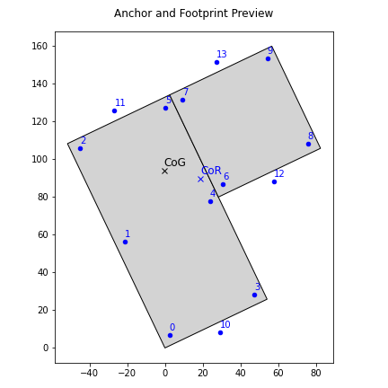
ezanchor.plotter.preview(equipment) preview anchor and footprint arrangement.
- equipment: ezanchor equipment object
- pass in your equipment analysis object
fig1 = eza.plotter.preview(AHU4)
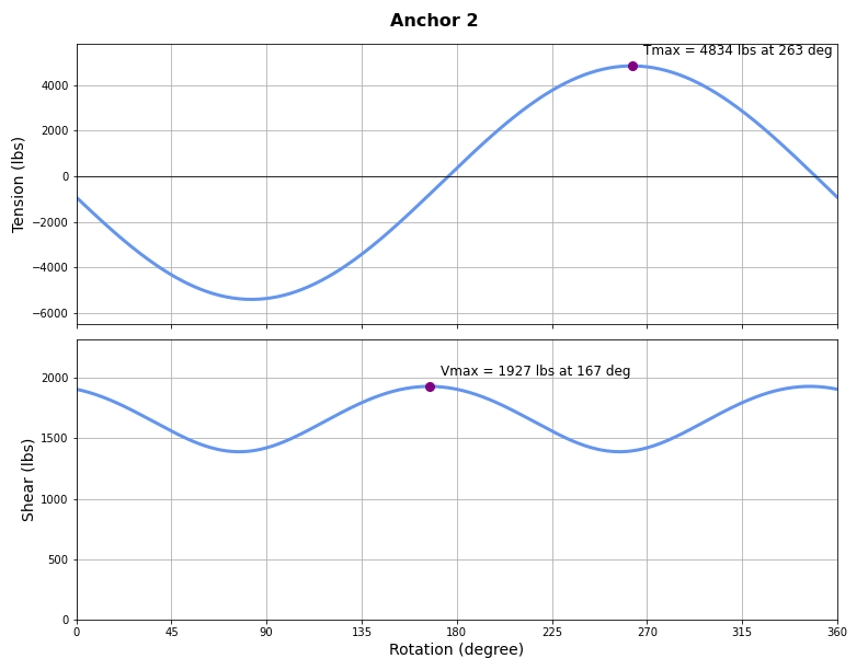
ezanchor.plotter.plot_anchor(equipment, anchorID) plot tension and shear in a specific anchor.
- equipment: ezanchor equipment object
- pass in your equipment analysis object
- anchorID: int
- specific anchor ID (use preview plot to see which anchor you are interested in)
fig2 = eza.plotter.plot_anchor(AHU4, 2)
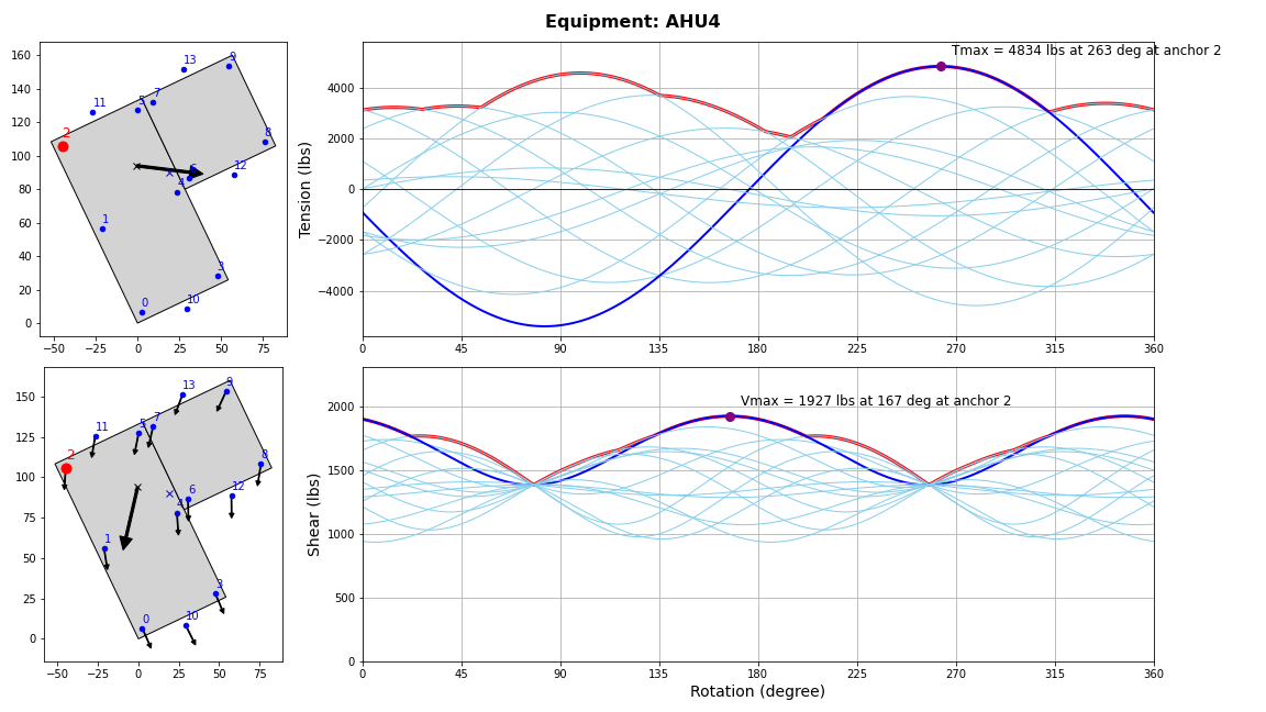
ezanchor.plotter.plot_equipment(equipment) plot tension and shear evenlope curve and other information.
- equipment: ezanchor equipment object
- pass in your equipment analysis object
fig3 = eza.plotter.plot_equipment(AHU4)
Step 6: Export results to CSV
Equipment.export_data() export results to csv file in the current working directory.
EZAnchor will create a folder called {Equipment.name}_run_results. Within this folder you will see two csv files.
AHU4_anchors.csv- results for individual anchorsAHU4_equipment.csv- results for equipment
AHU4.export_data()
Theoretical Background
Anchor Group Geometric Properties
An anchor group can be treated like an elastic section with geometric properties like centroid and moment of inertias. Unlike a cross-section, which has continuous area, anchors are assumed to have equal unitary area at discrete locations.
Centroid:
$$x_{COR} = \sum x_i / N_{anchors}$$
$$y_{COR} = \sum y_i / N_{anchors}$$
Moment of Inertias:
$$I_x = \sum (y_i - y_{COR})^2$$
$$I_y = \sum (y_x - x_{COR})^2$$
Polar Moment of Inertia:
$$J = I_x + I_y$$
Product Moment of Inertia:
$$I_{xy} = \sum(x_i - x_{COR})(y_i - y_{COR})$$
Angle to Principal Orientation:
$$\theta_p = 0.5 \times atan(\frac{I_{xy}}{2(I_x-I_y)})$$
Anchor Shear - Elastic Method
it is common to assume perfect alignment between anchor group COR and the component COM. In such cases, shear demand is simply the total horizontal force divided by the number of anchors.
$$V_i =F_h/N_{anchor}$$
In reality, COR and COM are often misaligned which produces additional shear demand due to in-plane torsion. The total shear demand is equal to direct shear plus an additional torsional shear.
$$V_i = V_{direct} + V_{torsion}$$
Direct shear in both orthogonal direction:
$$V_{direct,x} = -F_hcos(\theta) / N_{anchor}$$
$$V_{direct,y} = -F_h sin(\theta) / N_{anchor}$$
In-plane torsion is calculated as:
$$e_x = x_{COM} - x_{COR}$$
$$e_y = y_{COM} - y_{COR}$$
$$M_{torsion} = -F_hcos(\theta) e_y + F_hsin(\theta)e_x$$
Torsional shear is calculated as follows for an anchor located at $(x_i,y_i)$.
$$V_{torsion,x} = \frac{M_{torsion}(y_i - y_{COR})}{J}$$
$$V_{torsion,y} = \frac{M_{torsion}(x_i - x_{COR})}{J}$$
The resultant anchor shear is the sum of the terms above added together vectorially:
$$V_i = \sqrt{(V_{direct,x} + V_{torsion,x})^2 + (V_{direct,y} + V_{torsion,y})^2}$$
Anchor Tension - Elastic Method
Use this method by setting the on_stilt parameter to False. There are two major assumptions when we use the elastic method.
- Neutral axis coincides with the anchor group centroidal axis.
- Overturning moment is resolved entirely through the anchors without consideration of any bearing surface. Anchors are assumed to take compression, and must do so to maintain equilibrium.
Elastic method assumes that tension demand varies linearly, emanating from zero at the centroid outwards to the extreme fibers/anchors/legs.
Because anchors can theoretically take compression in this method, we have track the signs carefully. Let the vertical and horizontal force $F_v$ and $F_h$ always be positive. Negative signs are inserted where applicable to maintain right-hand convention.
Axial demand due to self-weight is simply the vertical force divided by the number of anchors.
$$P_{weight} = -F_v/N_{anchors}$$
Overturning moment due to horizontal force
$$M_{OT,x} = -F_h sin(\theta) \times Z_{COM}$$
$$M_{OT,y} = F_h cos(\theta) \times Z_{COM}$$
If weight is off-centered, there is an additional self-weight-induced overturning demand. This shifts the weight distribution such that $F_v$ is no longer evenly distributed amongst the anchors.
$$M_{weight,x} = -F_v (y_{COM} - y_{COR})$$
$$M_{weight,y} = F_v (x_{COM} - x_{COR})$$
The total overturning moment:
$$M_{total,x} = M_{OT,x} + M_{weight,x}$$
$$M_{total,y} = M_{OT,y} + M_{weight,y}$$
Axial demand due to overturning:
$$P_{Mx} = \frac{M_{total,x}(y_i - y_{COR})}{I_x}$$
$$P_{My} = \frac{M_{total,y}(x_i - x_{COR})}{I_y}$$
Apply principle of superposition to get the total anchor axial demand
$$P_i = P_{weight} + P_{Mx} + P_{My}$$
The equations above are only valid when the anchor group is in its principal orientation ($I_{xy}=0$).
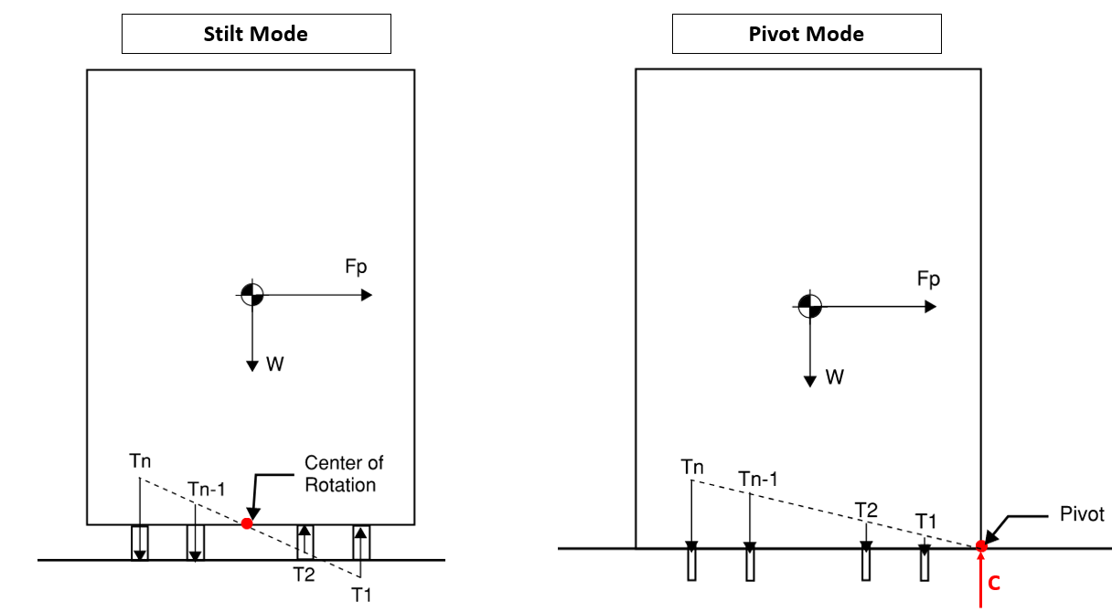
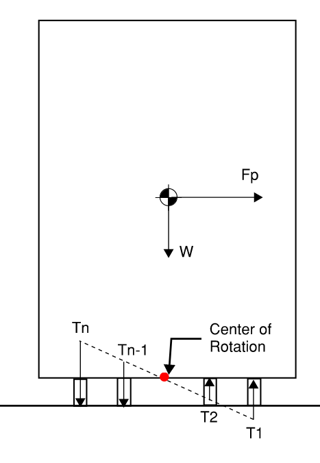
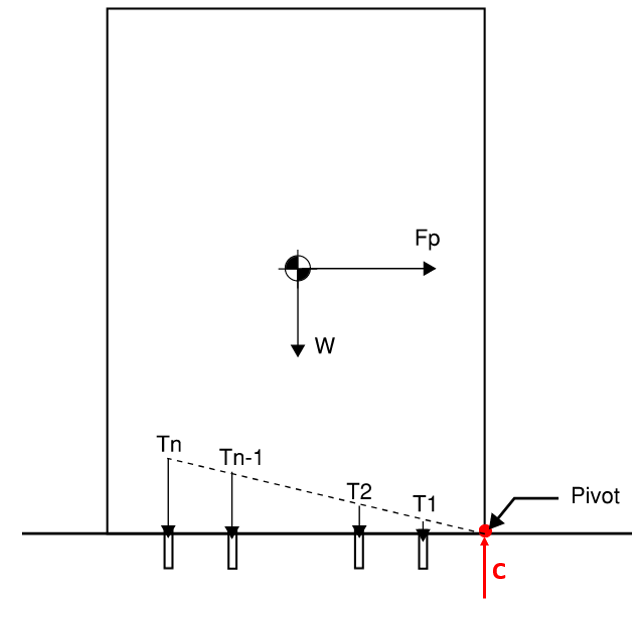
Anchor Tension - Rigid Base Method
Use this method by setting the on_stilt parameter to True. Here, we idealize the equipment as a rigid box with a fully rigid base.
As the component tips over, a linear strain profile is assumed along the base. Embedded in this method is an assumption of neutral axis depth, whose determination is a topic of considerable variability. EZAnchor takes the simplest approach of assuming axis of rotation to occur at the very edge of the component. In the figure below, notice how the bearing reaction (C) is a concentrated point load rather than a distributed load whose resultant lies some distance away from the edge.
In most cases, the depth of compression stress block is relatively small compared to the component footprint due to ample bearing area and low tensile capacity of concrete anchors. Nevertheless, It may be prudent to check if the component footprint is indeed large enough relative to the neutral axis depth.
The applied horizontal force induces an overturning moment:
$$M_{OT} = F_h \times Z_{COM}$$
The vertical force from the weight of the equipment induces a restoring moment that counteracts the overturning moment. $d_w$ is the distance between component center of mass, and the point of pivot which is assumed at the edge of the component.
$$M_R = F_v \times d_w$$
The net overturning moment is equal to:
$$M_{net} = M_{OT} - M_{R}$$
If $M_{net}$ is negative, then the component is not at risk of tipping over. Otherwise, tension demands are calculated by assuming a linear profile. Anchor furthest away from the neutral axis has the highest tension demand and is denoted $T_N$, For the other anchors:
$$T_i = \frac{d_i}{d_N}T_n$$
With this linear relationship established, use the moment equilibrium equation and solve for $T_n$
$$\sum M = 0 = -F_hZ_{COM} + F_vd_w + \sum T_i d_i$$
$$F_h Z_{COM} - F_v d_w = M_{net} = \sum (\frac{d_i}{d_N}T_n)d_i$$
$$M_{net} = \frac{T_n}{d_n}\sum (d_i)^2$$
$$T_n = T_{max} = \frac{M_{net} d_N}{\sum (d_i)^2}$$
Once we have $T_n$, use the linear relationship to determine $T_i$ (the intermediate anchors). Alternatively, we can just use the equation above for all anchors but just replace $d_N$ with $d_i$. Does it seem familiar? Looks like the elastic method just with the neutral axis shifted!
$$T_i = \frac{M_{net}d_i}{\sum (d_i)^2}$$
Lastly, the compression resultant can be calculated using force equilibrium:
$$C = F_v + \sum T_i$$
Notes and Assumptions
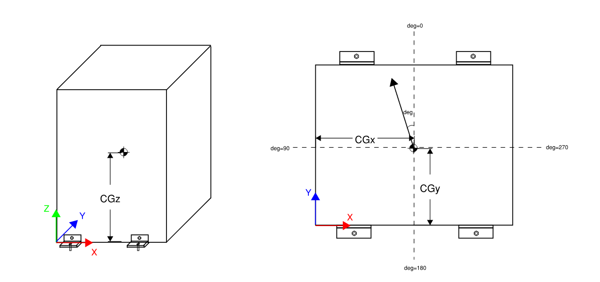
- Default coordinate system (X, Y, Z):
- Z is the vertical axis (Elevation)
- X and Y are the axes on plan. +X points to the right, +Y points up
- Sign convention:
- At degree 0, seismic load is applied in the +Y direction (upward) (don't ask me why I rotated 90 degrees. Makes no sense in retrospect. Ideally you should make +X the 0th degree so the cosines and sines just work)
- Sign of moment follows the right-hand rule. Mz is positive counter-clockwise
- Compression is negative (-), tension is positive (+)
- EZAnchor is agnostic when it comes to unit. Please ensure your input is consistent. I prefer to use lbs and inches
License
MIT License
Copyright (c) 2023 Robert Wang
Release history Release notifications | RSS feed


Download files
Download the file for your platform. If you're not sure which to choose, learn more about installing packages.
Source Distribution
Built Distribution
Filter files by name, interpreter, ABI, and platform.
If you're not sure about the file name format, learn more about wheel file names.
Copy a direct link to the current filters
File details
Details for the file ezanchor-1.1.0.tar.gz.
File metadata
- Download URL: ezanchor-1.1.0.tar.gz
- Upload date:
- Size: 26.6 MB
- Tags: Source
- Uploaded using Trusted Publishing? No
- Uploaded via: twine/6.1.0 CPython/3.11.0
File hashes
| Algorithm | Hash digest | |
|---|---|---|
| SHA256 |
350d28a8782783f9406d0f094789888ef6452f90d05638e3071b1856769eccd3
|
|
| MD5 |
193915a7b9d586e2ee9ed01ea24b83f7
|
|
| BLAKE2b-256 |
a471b7c712b46e4c99abca700527c5ebd6ecc54daecf842de31ffae653f17877
|
File details
Details for the file ezanchor-1.1.0-py3-none-any.whl.
File metadata
- Download URL: ezanchor-1.1.0-py3-none-any.whl
- Upload date:
- Size: 19.9 kB
- Tags: Python 3
- Uploaded using Trusted Publishing? No
- Uploaded via: twine/6.1.0 CPython/3.11.0
File hashes
| Algorithm | Hash digest | |
|---|---|---|
| SHA256 |
346021e68c573d8d9b97894c7ff6ff01b0cdd32cfd2caf3d124c0e74afb546a2
|
|
| MD5 |
8b0dc2ee51d78e1737c899cb66b53327
|
|
| BLAKE2b-256 |
22487ea1454c79a942bfed5ffc1f5bcec82e0e99f17769aa96012c8268233872
|


