ezweld - weld stress calculations in python

Project description

Weld Stress Calculation in Python
- Quick Start
- Validation Examples
- Installation
- Usage
- Theoretical Background
- Assumptions and Limitations
- License
Quick Start
Run main.py:
import ezweld
# initialize a weld group
weld_group = ezweld.WeldGroup()
# draw welds
weld_group.add_line(start=(0,0), end=(0,10), thickness=5/16)
weld_group.add_line(start=(5,0), end=(5,10), thickness=5/16)
# preview geometry
weld_group.preview()
# calculate weld stress (k/in) with elastic method
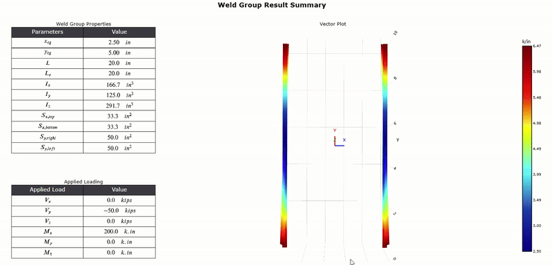
results = weld_group.solve(Vx=0, Vy=-50, Vz=0, Mx=200, My=0, Mz=0)
# plot results
weld_group.plot_results()
# plot results in 3D
weld_group.plot_results_3D()
Sign convention shown below:
weld_group.preview() returns a matplotlib figure showing what the weld group looks like and its geometric properties.
weld_group.solve() returns a pandas dataframe containing all the results.
weld_group.plot_results() returns a matplotlib 2D figure.
weld_group.plot_results_3D() returns interactive plotly 3D figure .
Validation Examples
Example 1: Two 8" vertical strips, separated by 6" width, subjected to Vy = -50 kips, and Mx = 120 k.in.
Hand calculation using elastic method and formulas in the Blodgett textbook:

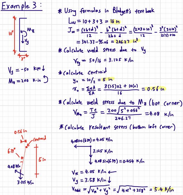
Results produced by ezweld matches hand calculation almost exactly.
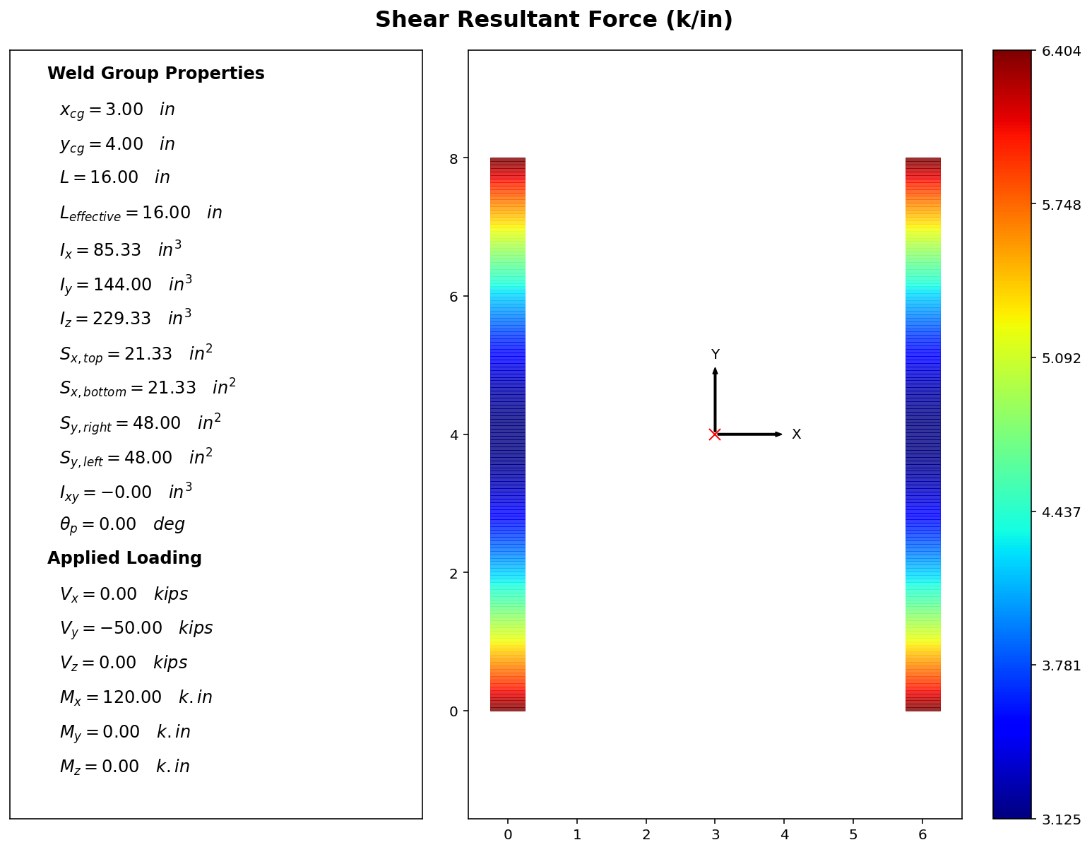
[!IMPORTANT] The small discrepancy (0.04 k/in) between numerical and theoretical result is due to how the weld group is discretized. Each fiber is 0.05" in length, and its associated stress is calculated at the centroid. Therefore, the top-most extreme fiber's centroid is actually 0.025" from the actual top. To improve numerical accuracy, the user may wish to set a smaller patch size.
Default patch size is 0.05". To set a smaller patch size, initialize the weld group with the PATCH_SIZE argument: weld_group = ezweld.WeldGroup(PATCH_SIZE=0.01).
In the example above, we know $I_x = 85.33 in^3$, $M_x = 120 k.in$, and if we use $c = (4 - 0.025) = 3.975$
$$v_{Mx} = Mc/I = 120(3.975)/85.33 = 5.59 k/in \quad \mbox{compared to 5.62 k/in theoretical}$$
$$v_{max} = \sqrt{(3.125)^2 + (5.59)^2} = 6.404 k/in \quad \mbox{compared to 6.435 k/in theoretical}$$
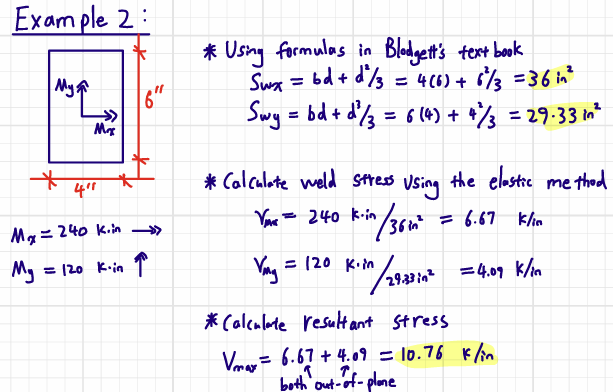
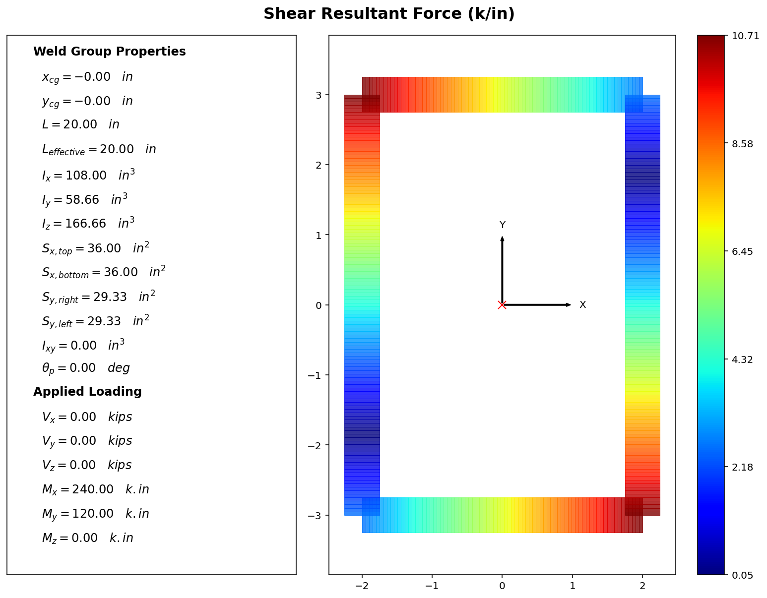
Example 2: A 6" x 6" rectangular weld, subjected to Mx = 240 k.in, and My = 120 k.in.
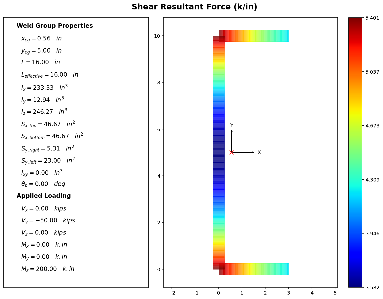
Example 3: A C-shaped weld 3" wide, 10" tall subjected to Vy = -50 kips, and Mz = 200 k.in
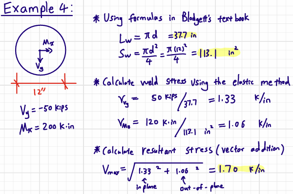
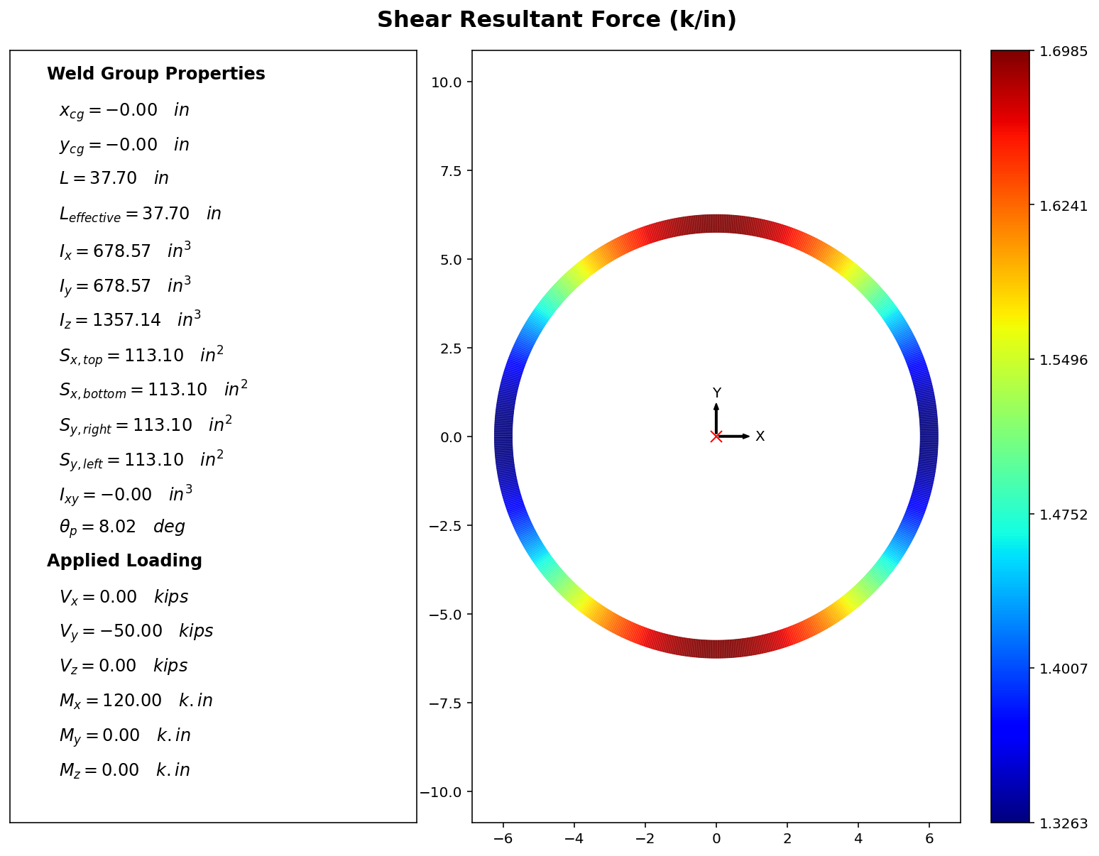
Example 4: A 12" diameter circular weld, subjected to Vy = -50 kips, and Mz = 120 k.in.
Installation
Option 1: Anaconda Python
Run main.py using your base Anaconda environment.
- Download Anaconda python
- Download this package (click the green "Code" button and download zip file)
- Open and run "main.py" in Anaconda's Spyder IDE.
The following packages are used:
- Numpy
- Pandas
- Matplotlib
- Plotly
Option 2: Regular Python
- Download this project to a folder of your choosing
git clone https://github.com/wcfrobert/ezweld.git - Change directory into where you downloaded ezweld
cd ezweld - Create virtual environment
py -m venv venv - Activate virtual environment
venv\Scripts\activate - Install requirements
pip install -r requirements.txt - run ezweld
py main.py
Pip install is also available.
pip install ezweld
Usage
Here are all the public methods available to the user:
Defining Weld Group
ezweld.WeldGroup.add_line(start, end, thickness)ezweld.WeldGroup.add_rectangle(xo, yo, width, height, thickness)ezweld.WeldGroup.add_circle(xo, yo, diameter, thickness)ezweld.WeldGroup.rotate(angle)
Solving
ezweld.WeldGroup.solve(Vx=0, Vy=0, Vz=0, Mx=0, My=0, Mz=0)
Visualizations
ezweld.WeldGroup.preview()ezweld.WeldGroup.plot_results(plot="force", colormap="jet", cmin="auto", cmax="auto")ezweld.WeldGroup.plot_results_3D(colormap="jet", cmin="auto", cmax="auto")
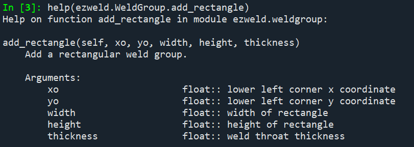
For more guidance and documentation, you can access the docstring of any method using the help() command.
For example, here's the output from help(ezweld.WeldGroup.add_rectangle)
Theoretical Background
Section Analogy
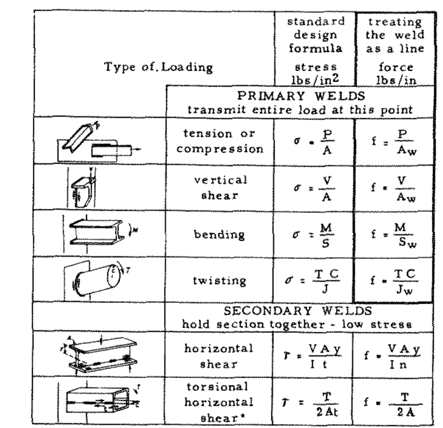
Welds enable force transfer between two connected members. At the plane of connection, we can think of the weld as the member itself; having its own geometric properties. With this assumption in mind, finding the stress state of a weld group is analogous to finding stress on a cross-section using the elastic stress formulas. Here is a figure from the “Design of Welded Structures” textbook by Omer W. Blodgett that illustrates this analogy.
First, we need to calculate the weld group's geometric properties. EZweld does so by discretizing the weld group into infinitesmially small patches to approximate the integral with summations.
Area:
$$A_w = \int_A dA = \sum t_i L_i$$
Centroid:
$$x_{cg} = \frac{\sum x_iA_i}{\sum A}$$
$$y_{cg} = \frac{\sum y_iA_i}{\sum A}$$
Moment of Inertia:
$$I_x = \int_A y^2 dA \approx \sum y_i^2A_i$$
$$I_y = \int_A x^2 dA \approx \sum x_i^2A_i$$
$$I_{xy} = \int_A xydA \approx \sum x_i y_i A_i$$
$$I_z = J = I_p = I_x + I_y$$
Section modulus:
$$S_{x,top} = \frac{I_x}{c_{y1}}$$
$$S_{x2,bot} = \frac{I_x}{c_{y2}}$$
$$S_{y,left} = \frac{I_y}{c_{x1}}$$
$$S_{y,right} = \frac{I_y}{c_{x2}}$$
Notations:
- $t_i$ = weld patch thickness
- $L_i$ = weld patch length
- $x_i$ = x distance from weld group centroid to weld patch
- $y_i$ = y distance from weld group centroid to weld patch
- $c_{y1}$ = y distance from weld group centroid to top-most fiber
- $c_{y2}$ = y distance from weld group centroid to bottom-most fiber
- $c_{x1}$ = x distance from weld group centroid to left-most fiber
- $c_{x2}$ = x distance from weld group centroid to right-most fiber
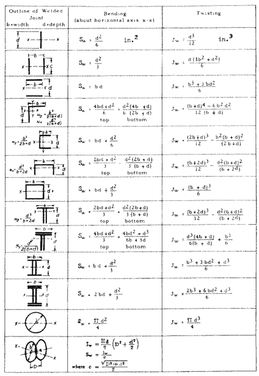
For common weld configurations, the section modulus ($S_w$) and polar moment of inertia ($J_w$) can be determined using the formulas below (from the Omer W. Blodgett textbook). Notice how the formulas have one dimensions less. We will discuss the use of force-per-unit-length convention in the next section.
$$x_{cg} = \frac{\sum x_iA_i}{\sum A}$$
$$y_{cg} = \frac{\sum y_iA_i}{\sum A}$$
Then, divide the weld group into individual line segments starting at $(x_1, y_1)$ and ending at $(x_2, y_2)$ with respect to the weld group centroid. The total moment of inertia can then be calculated using the equation below. The formula below comes from solving the line integral $\int x^2ds$ or $\int y^2ds$ for each line segment.
$$I_x = \sum \frac{t_i L_i}{3} (y_1^2 + y_1y_2 + y_2^2)$$
$$I_y = \sum \frac{t_i L_i}{3} (x_1^2 + x_1x_2 + x_2^2)$$
Force/Length Convention - Treating Welds as Lines
In the structural engineering context, welds are often thought of as 1-dimensional "lines". As such, results are often expressed as force per unit length (e.g. kip/in) rather than force per unit area (e.g. ksi). But why introduce another layer of complication when the stress formulas are completely fine?
Quoting Omer W. Blodgett's in his textbook first published in 1966. Chapter 2.2-8:
"[On the line approximation for determining section properties] With a thin section, the inside dimension is almost as large as the outside dimension; and, in most cases, the property of the section varies as the cubes of these two dimensions. This means dealing with the difference between two very large numbers. In order to get any accuracy, it would be necessary to calculate this out by longhand or by using logarithms rather than use the usual slide rule [emphasis mine]. To simplify the problem, the section may be treated as a line, having no thickness."
In other words, treating thin-sections with one dimension less was quite useful during the slide-rule era. Furthermore, in Chapter 7.4-7, Blodgett presents two other reasons for treating welds as lines which I will summarize here:
- With the line method, geometric properties, as well as demands can be calculated without specifying a thickness upfront. This is convenient from a workflow perspective because engineers can now calculate a demand, then specify a thickness afterwards. In the pre-calculator era when engineering calculations are not automated, change in the input parameter could mean revising pages of calculation by hand.
- Stress transformation and combination is burdensome to do by hand. The "force per unit length" convention is a design simplification that circumvents the thorny problem of stress transformations and change of basis.
Here are the exact same formulas as the previous section with one dimension less (set t = 1.0):
$$x_{cg} = \frac{\sum x_i L_i}{\sum L}$$
$$y_{cg} = \frac{\sum y_i L_i}{\sum L}$$
$$L_w = \iint dL = \sum L_i$$
$$I_x = \iint y^2 dL= \sum y_i^2 L_i$$
$$I_y = \iint x^2 dL = \sum x_i^2 L_i$$
$$I_{xy} = \iint xydL = \sum x_i y_i L_i$$
$$I_z = J = I_p = I_x + I_y$$
$$S_{x,top} = \frac{I_x}{c_{x1}}$$
$$S_{x2,bot} = \frac{I_x}{c_{x2}}$$
$$S_{y,left} = \frac{I_y}{c_{y1}}$$
$$S_{y,right} = \frac{I_y}{c_{y2}}$$
It is quite easy to convert between the two conventions (assuming uniform thickness within a weld group):
$$(ksi) = \frac{(k/in)}{t_{weld}}$$
$$(in^4) = (in^3)\times t_{weld}$$
In the rare case that a weld group has variable thickness, we must first calculate an "effective" length in proportional with the minimum thickness in the weld group, then use this effective length in the equations above. Be careful when using design equations provided in design tabls (such as the one above) as they often inherently assumes uniform thicknesses.
$$L_{effective,i} = \frac{t_i}{t_{min}} \times L_i$$
The resulting force must also be modified.
$$v_i\times(L_{effective,i} / L_i)$$
To show why this makes sense, Imagine two 10" lines of weld, one is 0.5" thick and another is 1" thick. We apply 100 kips shear. We get an uniform stress of (100 k / 15 in^2) = 6.66 ksi for both line of welds. However, notice that the 1" thick weld has 6.66 * 1 = 6.66 k/in whereas the 0.5" weld has 6.66 * 0.5 = 3.33 k/in. Checking equilibrium we have 66.6 kips + 33.3 kips = 100 kips.
Weld Stress Via Elastic Method
A weld group may be subjected to loading in all 6 degrees of freedom. These applied loads are then translated into stresses using the geometric properties above and the elastic stress formulas below.
Stress due to in-plane shear force ($V_x$, $V_y$):
$$v_{x,direct} = \frac{-V_x}{A_w}$$
$$v_{y,direct} = \frac{-V_y}{A_w}$$
Stress due to in-plane torsion ($torsion$):
$$v_{x,torsional} = \frac{torsion \times (y_i-y_{cg})}{J}$$
$$v_{y,torsional} = \frac{-torsion \times (x_i - x_{cg})}{J}$$
Stress from out-of-plane forces ($tension$, $M_x$, $M_y$):
$$v_{z,direct} = \frac{-tension}{A_w}$$
$$v_{z,Mx} = \frac{M_x (y_i-y_{cg})}{I_x}$$
$$v_{z,My} = \frac{M_y (x_i-x_{cg})}{I_y}$$
Sum the above terms together. Depending on the conventions used, these terms are either expressed as (force/length) or (force/area).
$$v_{x,total} = v_{x,direct} + v_{x,torsional}$$
$$v_{y,total} = v_{y,direct} + v_{y,torsional}$$
$$v_{z,total} = v_{z,direct} + v_{z,Mx} + v_{z,My}$$
For design purposes, the three terms above are combined into a single value and compared to a design capacity.
Resultant Unit Force - Simplified Approach
Using the "weld-as-line" convention (force/length), the three components above are simply added vectorially into a resultant shear force, then compared with an allowable unit shear capacity.
$$v_{resultant} = \sqrt{v_{x,total}^2 + v_{y,total}^2 + v_{z,total}^2} \leq \phi\frac{F_{EXX}}{\sqrt{3}}t_{weld} \approx \phi0.6F_{EXX}t_{weld}$$
Resultant Stress - Von-Mises Yield Criterion
Working with stress is trickier. The assumption of pure shear, and vector addition without stress transformation is convenient but not accurate. For example, complete-joint-penetration (CJP) welds and partial-joint-penetration (PJP) welds do have a normal stress component. Writing out the full Von-Mises yield criterion below, notice how the $\sigma$ term is not multiplied by 3, and thus $\sqrt{3}$ does not factor out cleanly.
$$\sigma_v = \sqrt{\frac{1}{2}[(\sigma_{xx}-\sigma_{yy})^2+(\sigma_{yy}-\sigma_{zz})^2+(\sigma_{zz}-\sigma_{xx})^2] + 3[\tau_{xy}^2+\tau_{yz}^2+\tau_{xz}^2]} \leq F_{EXX}$$
$$\sigma_v = \sqrt{\sigma_{zz}^2 + 3[\tau_{xy}^2+\tau_{yz}^2]}$$
For PJPs and CJPs, the Von-Mises stress is simple to calculate because we can easily distinguish what is normal stress and what is shear stress. The global vertical axis (Z) always aligns with the normal stress vector, and the global X and Y axes are the shear components. Therefore, the Von-Mises criterion for PJPs is calculated as follows.
$$\sigma_v = \sqrt{\tau_{z, total}^2 + 3[\tau_{x, total}^2+\tau_{y, total}^2]} \leq \phi F_{EXX}$$
Fillet welds introduce another layer of complexity because it actually has three failure planes. We typically assume failure to occur along the inclined throat (more info here). The elastic method derived above technically calculates the stresses at the horizontal face. We need to somehow map this to the diagonal face. The problem is we don't know which cartesian component (z' or y') becomes the normal component along this inclined axis. Do we rotate -45 degrees or +45 degrees? This is difficult to know without explicitly asking the user specify where the fillet weld face is pointing.
EZweld will assume conservatively that all stress terms are shear (i.e. multiple everything under the sqrt by 3). This matches the simplified unit-force approach above.
$$\sigma_v = \sqrt{3[\ \tau_{z, total}^2 + tau_{x, total}^2+\tau_{y, total}^2]} \leq \phi F_{EXX}$$
Fillet Weld Diagonal Failure Plane
To get the actual fillet weld stresses, we will need to use some linear algebra. First thing to note is that we are NOT looking at an infinitesmially small stress "cube" yet. Evaluation of fillet weld geometry is still a macro-level exercise.
First, we need to find a transformation matrix that maps force expressed in global coordinate system into force expressed in local coordinate system. The first transformation can be derived from the basis vectors of the local coordinate system, and the second transformation matrix is simply a rotation matrix about the local x-axis.
\{ v_{X}, v_{Y} , v_{Z} \} \rightarrow \{ p_{\perp}, v_{\parallel} , v_{\perp} \}
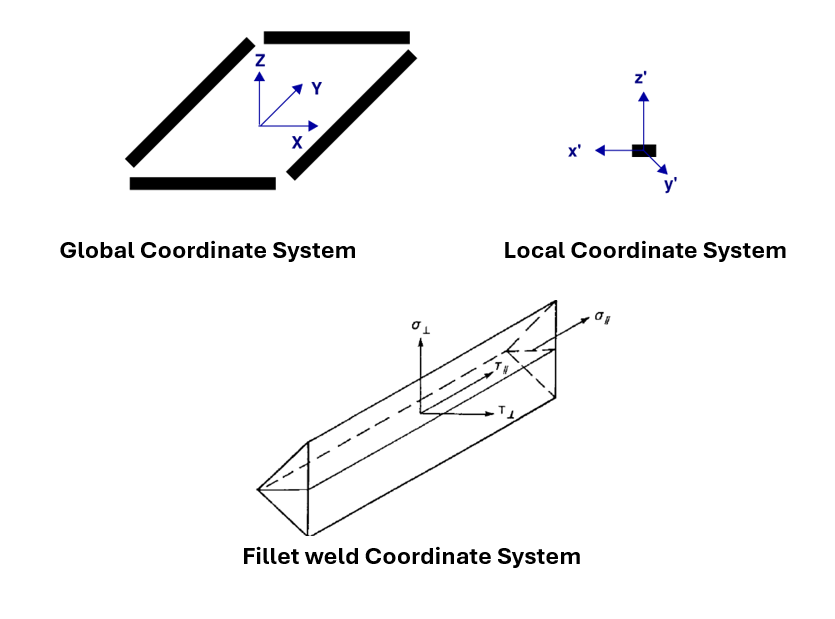
The longitudinal basis vector ($e_x$) is established by the start and end point of the weld line defined by the user.
u_{start}=\{x_i,y_i,0\}, \: u_{end}=\{x_i,y_i,0\}
$$e_x =\frac{u_{end} - u_{start}}{||u_{end} - u_{start}||} $$
Then we let the local basis vector ($e_z$) be exactly aligned with Z, which points upward.
e_z=\{0,0,1 \}
The last basis ($e_y$) is determined via a cross product. We crossed z' with x' to respect the right-hand convention. This vector indicates where the fillet weld face is located. If we were to walk from start node to end node, the fillet face will always be on the left.
$$e_y = \frac{e_z \times e_x}{||e_z \times e_x||} $$
The 3x3 geometric transformation matrix is defined by the x, y, and z basis vectors as the first, second, and third column, respectively.
$$ [T] = [e_x^T, e_y^T, e_z^T]$$
In addition, we want to apply a 45 degree rotation about the local x' axis:
$$ [R_{x}] = \begin{bmatrix} 1 & 0 & 0\ 0 & cos(45) & -sin(45)\ 0 & sin(45) & cos(45)\end{bmatrix} $$
Do a matrix multiplication with both $[T]$ and $[R_{x}]$ to get force expressed about the inclined local axis.The order of $[T]$ and $[R_{x}]$ is important here. We want rotations to apply "intrinsically".
\{ v_{\parallel}, v_{\perp} , n_{\perp}\} = [T][R_{x}] \{ v_{X}, v_{Y} , v_{Z} \}
Lastly, divide force by the throat area to get the stress.
Given the fact that most engineers in the US use the unit-force convention, I am reluctant to introduce extraneous input parameters and output results that might confuse people. Also, I'll probably get the implementation wrong. Hence, EZweld will assume conservatively that all stress terms are shear (i.e. multiple everything under the sqrt by 3). This matches the simplified unit-force approach above.
$$\sigma_v = \sqrt{3[\ \tau_{z, total}^2 + \tau_{x, total}^2+\tau_{y, total}^2]} \leq \phi F_{EXX}$$
Assumptions and Limitations
-
Sign convention follows the right-hand convention. right is +X, top is +Y, out-of-page is +Z
-
Be careful when specifying negative tension force (i.e. compression). Compression is often transferred through other mechanisms like bearing rather than through the weld itself.
-
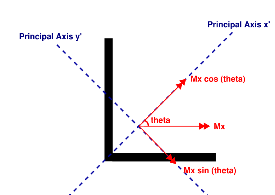
The combined stress formula is only valid when applied about a weld group's principal orientation. EZweld will automatically rotate the weld group if needed. In addition, remember to modify the applied moment into it components along the principal axes.
A weld group is in its principal orientation if the product of inertia is equal to zero:
$$I_{xy} = 0$$
Otherwise, the weld group must be rotated by the following angle.
$$\theta_p = 0.5\times tan^{-1}(\frac{I_{xy}}{I_x - I_y})$$
-
A key limitation of the elastic method is the assumption that no bearing surface exists. Consequently, out-of-plane moment must be resolved through the welds alone. This is done by assuming a very conservative neutral axis location that coincides with the weld group centroid, which means half of the weld fibers are put into compression to maintain equilibrium.
-
The elastic method does not take into account deformation compatibility and the effect of load angle. Welds are assumed to share loads equally under direct shear. In actuality, welds oriented transversely to applied loading have up to 50% higher capacity and stiffness (but lower ductility).
-
This is not enterprise-grade software. Please do NOT use it for work. Users assume full risk and responsibility for verifying that the results are accurate.
License
MIT License
Copyright (c) 2024 Robert Wang
Release history Release notifications | RSS feed


Download files
Download the file for your platform. If you're not sure which to choose, learn more about installing packages.
Source Distribution
Built Distribution
Filter files by name, interpreter, ABI, and platform.
If you're not sure about the file name format, learn more about wheel file names.
Copy a direct link to the current filters
File details
Details for the file ezweld-0.2.1.tar.gz.
File metadata
- Download URL: ezweld-0.2.1.tar.gz
- Upload date:
- Size: 4.3 MB
- Tags: Source
- Uploaded using Trusted Publishing? No
- Uploaded via: twine/6.0.1 CPython/3.13.1
File hashes
| Algorithm | Hash digest | |
|---|---|---|
| SHA256 |
5eaac61c127434a870a275b32e2be3b664d65fd618d662c52a4100ec07193001
|
|
| MD5 |
8ab3de9afd24d44bf963d731e982e123
|
|
| BLAKE2b-256 |
99217e521a79c0ddfc67ed13abaa7b76bcfcd98c677affaa14340ba7282c9e06
|
File details
Details for the file ezweld-0.2.1-py3-none-any.whl.
File metadata
- Download URL: ezweld-0.2.1-py3-none-any.whl
- Upload date:
- Size: 19.7 kB
- Tags: Python 3
- Uploaded using Trusted Publishing? No
- Uploaded via: twine/6.0.1 CPython/3.13.1
File hashes
| Algorithm | Hash digest | |
|---|---|---|
| SHA256 |
d9dfa65076c69b57a988d341e95c74d6f7369bd1402e18fec3a9da5169b399f3
|
|
| MD5 |
0df394626dcb2b4d855b47c89db79fd3
|
|
| BLAKE2b-256 |
b00e8c2e5acfe5c8d84faf91a67f38ebc36488d767f9ca26cbb80103d4c03724
|


