
Fannar

Representation spaces of trained models from Gram matrices of several sources of information: one positive-definite kernel per source, admissible transformations, Hadamard composition, and the geometry and spectral energy of the resulting matrix.
Fannar is the name of the method, and this library is its implementation. Both are described in the paper Building Spaces via Similarity Tensors in Reproducing Kernel Hilbert Spaces: A Mechanistic Interpretability Method.
Documentation: fannar.fernandocsdm.com/docs.
pip install fannar               # core: numpy + matplotlib
pip install "fannar[all]"        # + PyTorch, scikit-learn and pandas
pip install -e ".[test]"         # from this directory, for development
What it shows
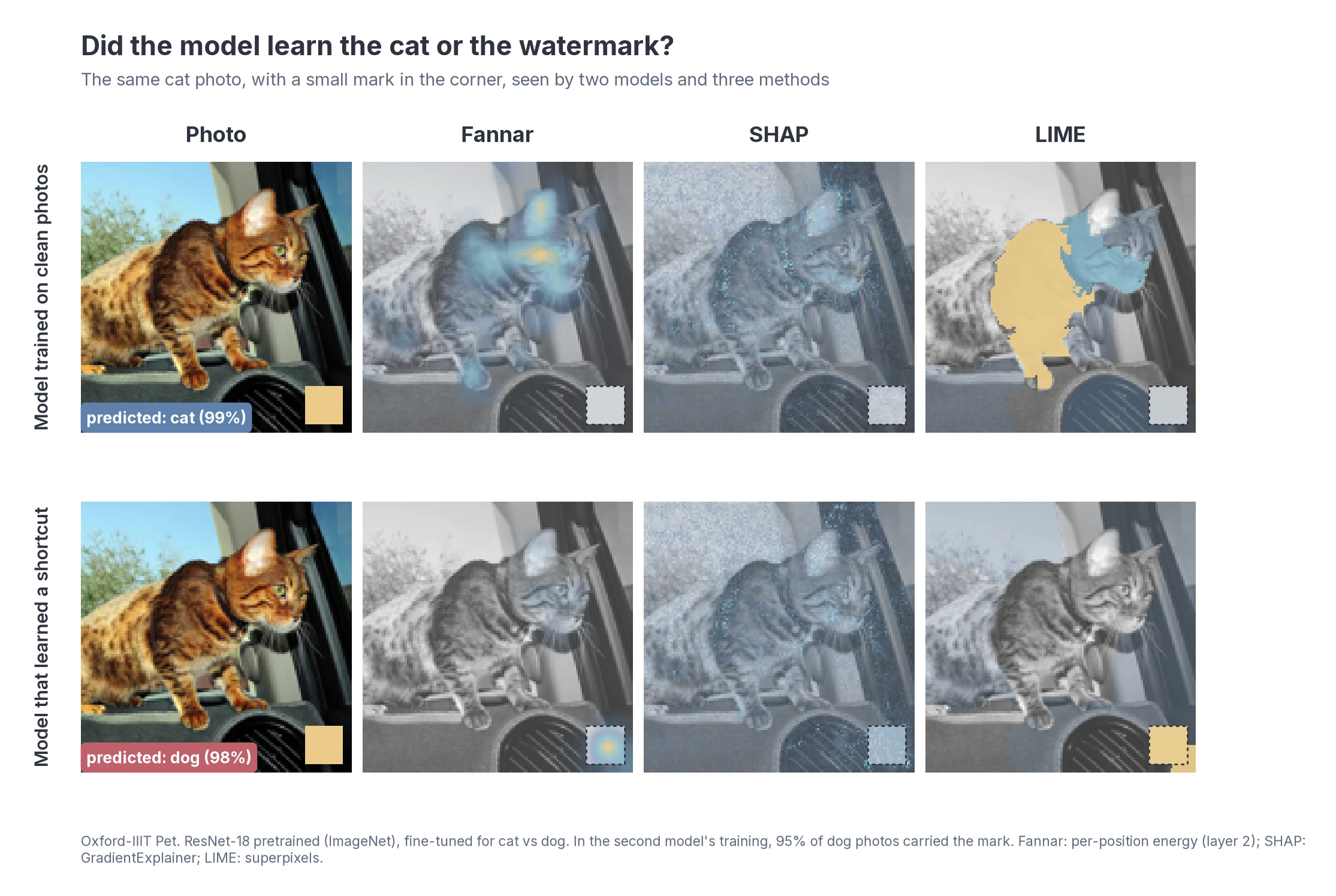
A ResNet-18 trained with a small mark on 95% of the dog photos learns the shortcut: it calls 40% of the marked cats dogs. In that model, half of Fannar's energy map falls on the mark, which covers 2% of the image. In the clean model, 91% falls on the animal.
 |
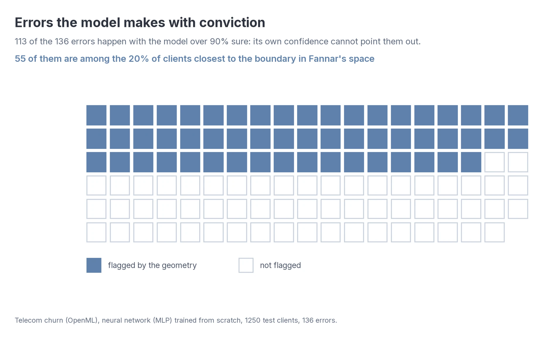 |
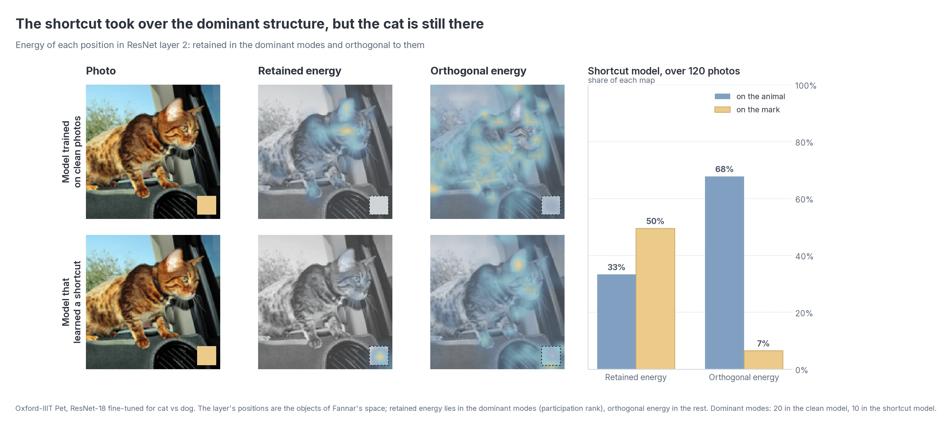
| Retained vs. orthogonal energy. The shortcut takes the dominant modes, but the cat is still represented outside them: 68% of the orthogonal energy sits on the animal. | Confident errors. 113 of the 136 errors of a churn network come with more than 90% confidence. The geometric margin flags 55 of them. |
 |
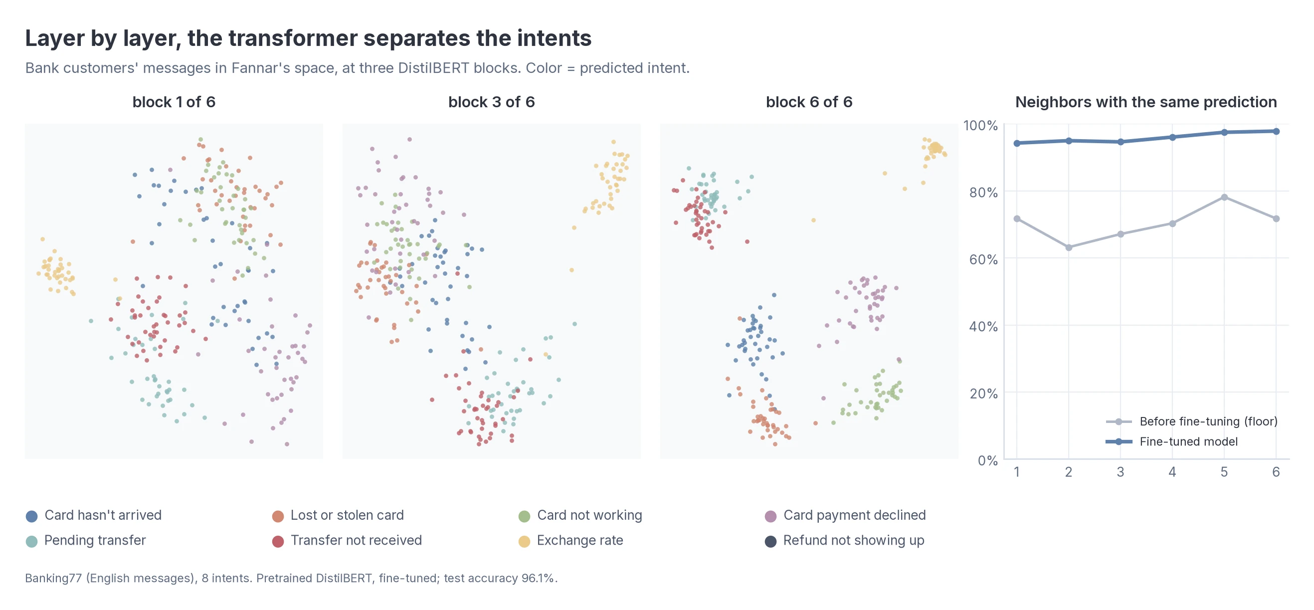 |
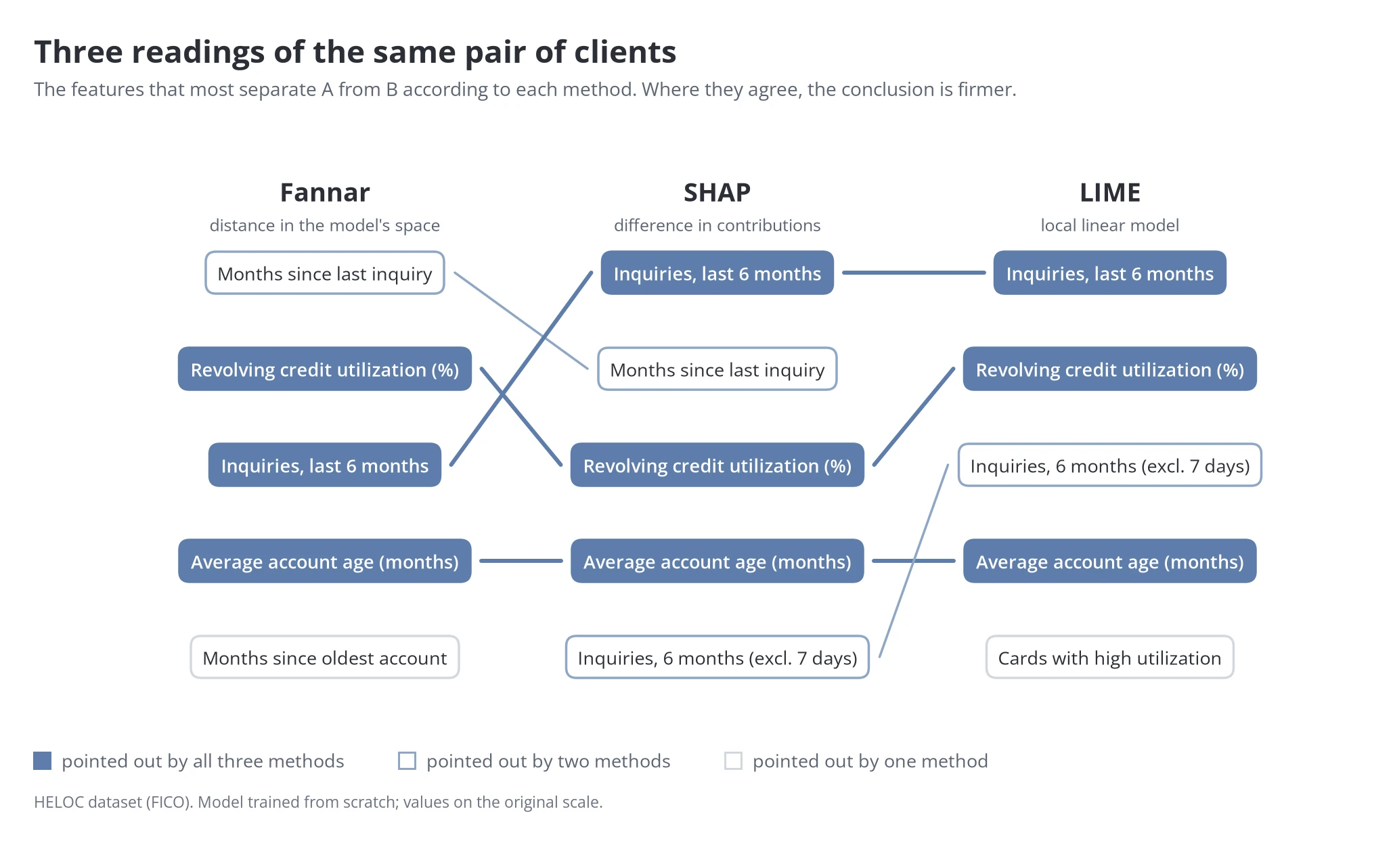
| Pair explanations (XGBoost). What separates a rejected applicant from a similar approved one. Where Fannar, SHAP and LIME agree, the conclusion is firmer. | Transformers. Customer intents separating block by block in a fine-tuned DistilBERT, against the same model before fine-tuning. |
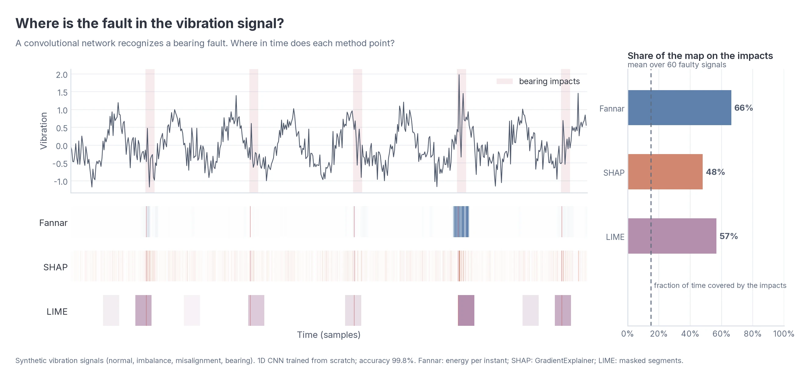
In time series, the per-instant energy of a 1D CNN concentrates on the impacts of a bearing fault: 66% of the map falls on them, and they cover 15% of the time.
These examples come from models trained to illustrate the method, one run each. The systematic evaluation is in the paper. More case studies, and the interpretability service, at fannar.fernandocsdm.com.
The idea in one line
G = T( T_1(K_1) ∘ T_2(K_2) ∘ … ∘ T_d(K_d) )
K_l is the raw Gram matrix of source l (from a kernel, or one you supply), T_l the
component transform, ∘ the Hadamard product and T the final transform. By the Schur product
theorem, G is positive semidefinite for any such choice. It therefore defines a geometry
(distances, neighbourhoods, level sets) and a spectral decomposition of energy.
The library keeps two things apart, as the paper does:
- the method: the construction above and the readings on
G(KernelPipeline,GramSpace); - the instantiation: which objects, which sources, which kernels and transformations
(
TorchSources,TreeSources, or a function of yours).
Quick start: a PyTorch model
import copy
import fannar as fa

initial = copy.deepcopy(model)        # keep it before training: it is the floor of the readings
# ... train `model` ...

interp = fa.Interpreter(
    model, X_test, y_test,            # the trained model and the objects to interpret
    layers=["layer1", "layer2", "layer3"],   # names from model.named_modules()
    reference_model=initial,          # optional: the floor (the same network at initialisation)
    feature_names=names,              # optional: for the pair explanations
)

report = interp.evaluate()            # readings per layer: joint, baselines and floor
print(report.to_markdown())           # also: report.to_frame(), report.to_json("r.json")

interp.plot_report(report)            # readings × layers
interp.plot_embedding()               # each layer's space in its two dominant modes
interp.plot_gram("layer2")            # components, Hadamard product and final Gram
interp.plot_spectrum("layer2")        # eigenvalues and participation rank

expl = interp.explain_pair(0)         # why does object 0 differ from its nearest neighbour
expl.top(5)                           #   with another prediction? [(feature, x_i, x_j, share)]
expl.plot()                           # each feature's share, layer by layer
interp.swap_test(50)                  # swap validation: method × |Δx| × random

emap = interp.energy_map(image, "layer2")   # CNN: retained energy at each position of the image
By default each layer provides three sources, as in the paper:
| source | what it is |
|---|---|
activations |
the layer's output, pooled to a common grid of positions |
gradients |
the derivative of the contrastive margin f_c − mean(f_{c'≠c}) with respect to that output |
parameters |
the filters the object activated, p[:, s] = Σ_c A[c, s] W[c, :] |
The default pipeline is "paper": a linear kernel, (T_a(K) + J)/2 on each component, the
Hadamard product, and T_tr ∘ T_c.
Two safeguards built into the code
- Gradient target. With
target="predicted", the gradient carries the prediction itself, and readings about the decision become circular. The default istarget="fixed"(classfixed_classfor every object). - Floor. Every reading needs a reference. Pass
reference_model(the same architecture with its initial weights). The report measures that network's geometry against the trained network's behaviour, so the only difference between a reading and its floor is training.
One module per kind of data
Since 0.4.0, each kind of data has its own entry point. Each one is an Interpreter with suitable
defaults and the same methods, and gives the same numbers as fa.Interpreter with the same
options. The modules load on first access, so import fannar stays light.
import fannar as fa

fa.tabular.TabularInterpreter(model, df_test, y_test, layers=[...])  # PyTorch on tables; the DataFrame gives the names
fa.image.ImageInterpreter(cnn, loader, y_test, layers=[...])         # CNN/ViT, (N, C, H, W) outputs, grid=4
fa.text.TextInterpreter(fa.text.wrap_hf(hf_model, pad_token_id=0), input_ids, y)  # transformers over tokens
fa.tree.TreeInterpreter(tree, df_test, y_test, X_train=df_train)     # scikit-learn tree, slack in standard deviations
| module | for | what it adds |
|---|---|---|
fannar.tabular |
PyTorch models over rows of features | takes a DataFrame/Series: feature and class names |
fannar.image |
CNNs and ViTs | grid=4, DataLoader input, energy maps per position |
fannar.text |
transformers over token sequences | layout="tokens", grid=8, wrap_hf, layers = encoder blocks |
fannar.tree |
scikit-learn decision trees | slack scale from X_train, labels of any type |
Examples
They all run offline in seconds, on datasets that ship with scikit-learn or on synthetic data
(pip install "fannar[all]", then python examples/<script>.py):
| script | module | what it shows |
|---|---|---|
quickstart_digits.py |
fannar.tabular |
the full tour: report, plots, pairs, swap test |
tabular_wine.py |
fannar.tabular |
DataFrame and categorical labels, pairs and errors |
tree_wine.py |
fannar.tree |
depths as layers, text labels, a tree as the floor |
image_digits_cnn.py |
fannar.image |
DataLoader input, energy map of one image |
text_keywords.py |
fannar.text |
wrap_hf, automatic layers, energy per token in each block |
custom_gram.py |
fannar |
your own sources, kernels and Gram matrices, no model |
Your own Gram matrix
Any component can come from a kernel of yours, a transform of yours, or a matrix you have already computed:
pipe = fa.KernelPipeline(
    {
        "state":  fa.Component(fa.Linear(), fa.angular() >> fa.shift(1.0)),
        "text":   fa.Component(fa.RBF(gamma=0.1), fa.identity),
        "mine":   fa.Component(lambda A, B: (A @ B.T + 1) ** 2),     # any function k(X, Y)
    },
    final=fa.center >> fa.trace_normalize,
)
space = pipe(sources={"state": S, "text": T, "mine": M}, labels=y)
space = pipe(grams={"state": K1, "text": K2, "mine": K3})           # ready-made matrices
space = fa.GramSpace(my_psd_matrix, labels=y)                      # or a G of your own, directly
Available transforms (they compose with >>, left to right): identity, center,
trace_normalize, frobenius_normalize, max_eig_normalize, angular(), shift(c),
whiten(), spectral(f), psd_project(). Kernels: Linear, Cosine, RBF, Polynomial,
FunctionKernel. Presets: fa.paper_pipeline(), fa.single_source("activations"),
fa.positions_pipeline().
With Gaussian kernels, the Hadamard product becomes exactly a sum of the sources' metrics (the product of Gaussians is the Gaussian of the sum of the exponents). To keep the multiplicative interaction between sources, prefer
Linear/Cosine.
The representation space (GramSpace)
space.distances               # pseudometric d(i,j)² = G_ii + G_jj − 2 G_ij
space.neighbors(i, k)         # k nearest neighbours
space.level_band(i, r, delta) # level band Γ_{r,δ}(i)
space.equivalence_classes()   # objects this space cannot tell apart
space.participation_rank()    # (tr G)² / ‖G‖²_F, without a spectral decomposition
space.energies()              # E_∥, E_⊥ and E_ratio per object
space.containment(labels)     # class directions inside V_r (r = K − 1)
space.embedding(2)            # coordinates in the two dominant modes (kernel PCA)
space.cka(other)              # centred alignment
space.decompose(K)            # G = a·K + R: what K explains, and the residual
Other models
# scikit-learn decision tree: path, slack and class distribution per depth
interp = fa.Interpreter(tree, X_test, y_test)          # or fa.tree.TreeInterpreter, above

# any model: a function returning {layer: {source: array}} and the predictions
def sources(X):
    return {"output": {"proba": model.predict_proba(X), "leaves": model.apply(X)}}, model.predict(X)

interp = fa.Interpreter(model, X_test, y_test, extractor=sources,
                        pipeline=fa.KernelPipeline(["proba", "leaves"]), baselines={})
Report readings
| reading | question |
|---|---|
knn_prediction |
do an object's neighbours share its prediction? |
correctness_auc |
does the geometric margin anticipate where the model errs? |
confusion_agreement |
are the classes the model confuses close to each other? (≥ 5 classes) |
containment |
are the class directions inside the retained subspace? |
e_ratio_error_auc |
does the energy outside the retained subspace flag the errors? |
Cost
Per Gram matrix, Θ(n²D + n³) with the full spectral decomposition (n objects, D the total
dimension of the sources). The participation rank takes Θ(n²). A pair explanation costs one
forward and one backward pass over F + 2 rows, linear in the number of features F.
Tests
pip install -e ".[test]" && pytest
Documentation
The documentation site lives in docs/lib/ (Markdown, MkDocs Material), and the API reference is
generated from the docstrings. It is published at fannar.fernandocsdm.com/docs by the portfolio
project, which serves the static files:
pip install -e ".[docs]"
mkdocs serve                        # preview at http://127.0.0.1:8000/docs/
bash scripts/publish_docs.sh        # build and copy to ../Portfolio/public/fannar/docs
Then commit and deploy the portfolio.
License
This work is licensed under a Creative Commons Attribution-NonCommercial 4.0 International License.

The full text is in LICENCE. For
commercial use of the method, see the interpretability service at
fannar.fernandocsdm.com.
1 maintainer

Metadata
1 maintainer
Release files for fannar 0.4.0
For a detailed explanation of source distributions (sdists) and built distributions (wheels), please see the package formats documentation.
Source distribution (sdist)
| File | Size | Uploaded | Provenance | Actions |
|---|---|---|---|---|
| fannar-0.4.0.tar.gz | 61.6 kB | With provenance | Details for fannar-0.4.0.tar.gz |
Built distribution (wheel)
| File | Interpreter | ABI | Platform | Actions Reset |
|---|---|---|---|---|
| fannar-0.4.0-py3-none-any.whl | Python 3 | none | any | Details for fannar-0.4.0-py3-none-any.whl |
Total release size: 119.9 kB
Release files / fannar-0.4.0.tar.gz
| Download URL | fannar-0.4.0.tar.gz |
|---|---|
| Size | 61.6 kB |
| Tags | Source |
|
SHA-256 checksum How to use checksums |
9ad7489f27b146b26121a9e3eb8f77166314cf6cef2f543ac8714d532f2ddd94
|
|
BLAKE2b-256 checksum How to use checksums |
190c2db97650bb8b8c9c33ffb750fd533a8dafd0d94bf9ba8724e93daaa99897
|
| Upload date | |
|
Uploaded using Trusted Publishing? What is trusted publishing? |
Yes |
| Uploaded via |
twine/7.0.0 CPython/3.13.16
|
Provenance
Provenance describes where a file came from. On PyPI, provenance is shared via attestations, which provide a verifiable record of the build or publishing details. View details, limitations and caveats.


PyPI Publish Attestation
PyPI verified that this artifact, at this checksum, originated from the publisher listed below.
Signed by GitHub Actions, verified by PyPI on Nov 16, 2026.
Transparency logRelease files / fannar-0.4.0-py3-none-any.whl
| Download URL | fannar-0.4.0-py3-none-any.whl |
|---|---|
| Size | 58.3 kB |
| Tags | Python 3 |
|
SHA-256 checksum How to use checksums |
6499bae05abf521b0c3c4ff1247793c552d97ca468cfce0d4d476d6495c41a7e
|
|
BLAKE2b-256 checksum How to use checksums |
150be8e21adfe1840c25be43eac976af3590eeab5757c8ee47d6252ad7945328
|
| Upload date | |
|
Uploaded using Trusted Publishing? What is trusted publishing? |
Yes |
| Uploaded via |
twine/7.0.0 CPython/3.13.16
|
Provenance
Provenance describes where a file came from. On PyPI, provenance is shared via attestations, which provide a verifiable record of the build or publishing details. View details, limitations and caveats.
PyPI Publish Attestation
PyPI verified that this artifact, at this checksum, originated from the publisher listed below.
Signed by GitHub Actions, verified by PyPI on Nov 16, 2026.
Transparency logSecurity for fannar 0.4.0
Provenance
Provenance describes where a file came from. On PyPI, provenance is shared via attestations, which provide a verifiable record of the build or publishing details. View details, limitations and caveats.
Full provenance
Both files in this release have been uploaded with provenance metadata.
Attestation for fannar-0.4.0.tar.gz
PyPI Publish Attestation
PyPI verified that this artifact, at this checksum, originated from the publisher listed below.
Signed by GitHub Actions, verified by PyPI on Nov 16, 2026.
Transparency logA note on package security
PyPI is a repository for distributing packages, not a service for auditing them. While third-party security researchers and our staff do their best to detect and remove malicious packages, PyPI cannot guarantee the quality, security or suitability of any given package.
To learn more about protecting yourself from malicious actors, visit our package security documentation.














