fapp (frame analysis program in python) is a simple, easy-to-use implementation of the direct stiffness method.

Project description

Frame Analysis Program in Python
A lightweight and easy-to-use Python implementation of the Finite Element Method (FEM). Perform first-order elastic analyses of any 3-D frame structure and visualize results with a fully interactive web browser interface.
Introduction
fapp, pronounced "F - app", stands for Frame Analysis Program in Python. As the name suggests, only line elements are currently supported (no surface or solid elements).
- Analyze any 3-D frame structures
- Timoshenko beam elements with shear deformation
- First-order elastic analyses
- Nodal and uniform member loads
- Imposed displacements
Features are somewhat limited in its current implementation but I'm sure you'll find it satisfactory for most basic use cases in structural engineering. The entire code base is only around 500 lines (not counting comments and the plotting functionalities). It was a joy to develop and I hope you'll love how simple it is to use!
I made a conscious effort to keep things pedagogically clear and concise during development. I hope it will serve as excellent reference material for educators looking for a python implementation of the direct stiffness method.
The underlying theory, procedure, and notations are explained in the textbook "Matrix Structural Analysis, 2nd Edition" by William McGuire, Richard Gallagher, and Ronald Ziemian. You can get a free PDF copy here: https://digitalcommons.bucknell.edu/books/7/. The object-oriented design of fapp is partly inspired by my Graduate school matrix analysis course project taught by Professor Gregory Deierlein, where we had to implement something similar in MATLAB. I also relied on several other free online resources such as COMSOL documentation for shape functions, and Professor Henri Gavin's course reader for stiffness matrix of a Timoshenko beam. These references available as pdfs in the \doc folder.
Disclaimer: this package is meant for personal or educational use only. As evident from the empty "\tests" folder, fapp is NOT robust enough to be used for commercial purposes of any kind! There are plenty of edge cases that I simply haven't had the time to explore/debug.
Quick Start
Installation
See "Installation" section below for more info. For casual users, simply use Anaconda Python, download this module, and open "main.py" in Spyder IDE.
Using fapp
# import fapp
import fapp.analysis as fpa
import fapp.plotter as fpp

# initialize structure
my_structure = fpa.Analysis()

# define nodes
my_structure.add_node(node_tag=0, x=0, y=0, z=0)
my_structure.add_node(node_tag=1, x=0, y=4000, z=0)
my_structure.add_node(node_tag=2, x=12000, y=7000, z=0)
my_structure.add_node(node_tag=3, x=12000, y=0, z=0)

# define elements
my_structure.add_element(ele_tag=0, i_tag=0, j_tag=1, A=2e4, Ayy=2e4, Azz=2e4, Iy=999, Iz=1.5e9, J=999, E=200, v=0.3, beta=0)
my_structure.add_element(ele_tag=1, i_tag=1, j_tag=2, A=4e4, Ayy=4e4, Azz=4e4, Iy=999, Iz=3.8e9, J=999, E=200, v=0.3, beta=0)
my_structure.add_element(ele_tag=2, i_tag=2, j_tag=3, A=2e4, Ayy=2e4, Azz=2e4, Iy=999, Iz=1.5e9, J=999, E=200, v=0.3, beta=0)

# define fixity
my_structure.add_fixity(node_tag=0, ux=0, uy=0, uz=0, rx=0, ry=0, rz=0)
my_structure.add_fixity(node_tag=3, ux=0, uy=0, uz=0)

# define loading
my_structure.add_load_member(ele_tag=1, wx=-0.00363, wy=-0.01455, wz=0)
my_structure.add_load_nodal(node_tag=1, Fx=5, Fy=0, Fz=0, Mx=0, My=0, Mz=0)

# start analysis
my_structure.solve()

# visualize results
fig1 = fpp.plot(my_structure)
fig2 = fpp.plot_results(my_structure, display="d")
fig3 = fpp.plot_diagrams(my_structure, ele_tag=0)
fig1.show()
fig2.show()
fig3.show()
Installation
Option 1: Anaconda Python Distribution
For the casual users, using the base Anaconda Python environment is recommened. This is by far the easiest method of installation. Users don't need to worry about dependency management and setting up virtual environments. The following open source packages are used in this project:
- Numpy
- Scipy
- Plotly
Installation procedure:
- Download Anaconda python
- Download this package (click the green "Code" button and download zip file)
- Open and run "main.py" in Anaconda's Spyder IDE. Make sure working directory is correctly configured.
Option 2: Command Prompt + Plain Python
- Download this project to a folder of your choosing
git clone https://github.com/wcfrobert/fapp.git - Change directory into where you downloaded fapp
cd fapp - Create virtual environment
py -m venv venv - Activate virtual environment
venv\Scripts\activate - Install requirements
pip install -r requirements.txt - run fapp
py main.py
Note that pip install is available.
pip install fapp
Usage
Step 0: Instantiate analysis object
fapp has an object-oriented design that is quite intuitive to understand and use. Start by instantiating an "Analysis" object. All your results and information related to the structure will be stored here.
import fapp.Analysis

my_structure = fapp.analysis.Analysis()
Step 1: Add nodes
Analysis.add_node(node_tag, x, y, z) adds a node to the structure. Parameters:
- node_tag: int
- Node tag must be defined chronologically from 0 to N. Node 0 will have DOF [0,1,2,3,4,5], node 1 will have DOF [6,7,8,9,10,11], and so on...
- x: float
- x coordinate
- y: float
- y coordinate
- z: float
- z coordinate
Add nodes to your structure with ".add_node" method. Please note node tag must be defined chronologically from 0 to N. This is because all node objects are stored in a list and its tag should correspond to its index. Furthermore, degree of freedoms (DOFs) are numbered chronologically for ease of implementation(also known as the plain numberer). It would have been simple enough to add a mapping step such that the node tag (used to determine DOF) is decoupled from a user-specified label, but that adds a layer of obfuscation that I was not particularly fond of.
# named arguments recommended for clarity
my_structure.add_node(0, 10, 0, 0)
my_structure.add_node(node_tag=1, x=0, y=0, z=0)

# nodes must be defined chronologically starting at 0. THe following is NOT allowed:
my_structure.add_node(node_tag=1, x=0, y=0, z=0) # ERROR! Must start from 0!
my_structure.add_node(node_tag=999, x=0, y=0, z=0) # ERROR! Second node so tag = 1
Step 2: Add elements
Analysis.add_element(ele_tag,i_tag,j_tag,A,Ayy,Azz,Iy,Iz,J,E,v=0.3,beta=0) adds an element to the structure. Parameters:
- ele_tag: int
- Element tag must be defined chronologically from 0 to N
- i_tag: int
- Start node tag
- j_tag: int
- End node tag
- A: float
- Section area
- Ayy: float
- Shear area along y axis (major bending direction). Input very large value to neglect shear deformation
- Azz: float
- Shear area along z axis (minor bending direction). Input very large value to neglect shear deformation
- Iy: float
- Moment of inertia about y axis (minor bending direction)
- Iz: float
- Moment of inertia about z axis (major bending direction)
- J: float
- Torsion constant
- E: float
- Young's modulus
- v: float (optional)
- Poisson's ratio. Default = 0.3. Used to determine shear modulus $G = \frac{E}{2(1+v)}$
- beta: float (optional)
- Member rotation along its longitudinal axis in degrees. Default = 0. Refer to "Notes and Assumptions" section for default geometric transformation
Once all the nodes have been defined, create elements by linking nodes together. In this step, we are defining both the connectivity as well as section/material properties. Again, element tag must be defined chronologically from 0 to N.
# Named arguments recommended for clarity
my_structure.add_element(0, 0, 1, 2e4, 2e4, 2e4, 999, 1.5e9, 999, 200, 0.3, 0)
my_structure.add_element(ele_tag=1, i_tag=1, j_tag=2, A=4e4, Ayy=4e4, Azz=4e4,
                         Iy=999, Iz=3.8e9, J=999, E=200, v=0.3, beta=0)
Step 3: Add fixity
Analysis.add_fixity(node_tag, ux="nan", uy="nan", uz="nan", rx="nan", ry="nan", rz="nan") adds fixity to the structure. Parameters:
- node_tag: int
- Node you wish to fix
- ux: int, float, string (optional)
- Displacement in global X direction. Default = "nan"
- uy: int, float, string (optional)
- Displacement in global Y direction. Default = "nan"
- uz: int, float, string (optional)
- Displacement in global Z direction. Default = "nan"
- rx: int, float, string (optional)
- Rotation about global X axis. Default = "nan"
- ry: int, float, string (optional)
- Rotation about global Y axis. Default = "nan"
- rz: int, float, string (optional)
- Rotation about global Z axis. Default = "nan"
Apply boundary conditions. You may wish to fix a node, or impose a prescribed displacement. Enter 0 for fixed, "nan" for free, float for prescribed displacement.
# fully fixed support
my_structure.add_fixity(node_tag=0, ux=0, uy=0, uz=0, rx=0, ry=0, rz=0)

# pin support. Note you only need to specify DOFs to fix. "nan" is default input
my_structure.add_fixity(node_tag=3, ux=0, uy=0, uz=0)

# fix displacement in X, Y, Z and rotation about X and Y. 2D pin if modeling in XY plane
my_structure.add_fixity(node_tag=4, ux=0, uy=0, uz=0, rx=0, ry=0)
Step 4: Add Loading
Analysis.add_load_member(ele_tag, wx=0, wy=0, wz=0) adds uniform load to a member. Defined with respect to its local axis. Parameters:
- ele_tag: int
- Element tag to identify element you wish to load
- wx: float (optional)
- uniform load along member local x axis. Axial direction. Default = 0
- wy: float (optional)
- uniform load along member local y axis. Major bending direction. Don't forget to put negative number for gravity load. Default = 0
- wz: float (optional)
- uniform load along member local z axis. Minor bending direction. Default = 0
# apply uniform load of -0.015 to element 1 in its local y axis
my_structure.add_load_member(ele_tag=1, wy=-0.015)
Analysis.add_load_nodal(node_tag, Fx=0, Fy=0, Fz=0, Mx=0, My=0, Mz=0) adds external nodal load. Defined with respect to global axis. Parameters:
- node_tag: int
- Node tag to identify node you wish to load
- Fx: float (optional)
- Nodal load in global X direction. Default = 0
- Fy: float (optional)
- Nodal load in global Y direction. Default = 0
- Fz: float (optional)
- Nodal load in global Z direction. Default = 0
- Mx: float (optional)
- Concentrated moment about global X axis. Default = 0
- My: float (optional)
- Concentrated moment about global Y axis. Default = 0
- Mz: float (optional)
- Concentrated moment about global Z axis. Default = 0
# Apply nodal load of 5.5 to node 1 in global X direction
my_structure.add_load_nodal(node_tag=1, Fx=5.5)
Step 5: Solve And Post-Process
Analysis.solve(print_info=True) starts analysis routine.
- print_info: Boolean (optional)
- Set to False if you do not want anything printed to terminal
The beauty of fapp's object-oriented design is that all the information related to the structure, from geometry, connectivity, to force/displacement results will be stored in one variable. The "Analysis" object doubles as a factory and stores a list of "Node" objects and "Element" objects. You can use dot notation to access everything. For example:
# retrieve x,y,z coordinate of node 2
my_structure.node_list[2].coord

# view the stiffness matrix of element 0
my_structure.element_list[0].k_local

# view nodal displacement at node 6 (after solving)
my_structure.node_list[6].disp
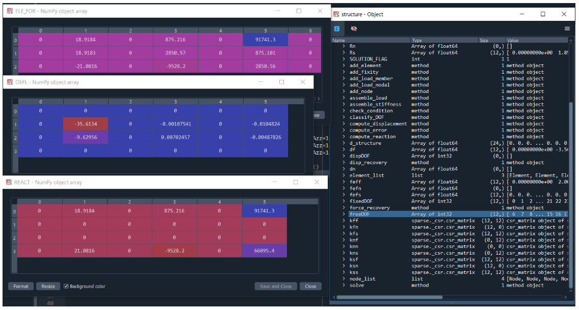
For ease of access, results are also collected and stored in matrices.
# N_node x 6 matrix containing nodal displacements
my_structure.DEFL
# N_node x 6 matrix containing reaction forces at fixed nodes
my_structure.REACT
# N_element x 12 matrix containing member-end forces in local coordinate
my_structure.ELE_FOR
# for example, return nodal displacement at node 3
my_structure.DEFL[3, :]
Spyder IDE's variable explorer is highly recommended!
Step 6: Visualize
To help with debugging, I built a visualization engine in Plotly. It allows the user to zoom, pan, orbit, and hover over nodes and elements for more information. All in a fully interactive web browser environment. I also added some camera buttons to help user switch between views.
There are currently three visualization options:
- plot() - for visualizing geometry, node and element tags, and connectivity
- Node hoverinfo shows tag, xyz coordinate, fixity, and loading
- Element hoverinfo shows tag, start and end node, length, member loading, and member rotation
- plot_result() - for visualizing results after analysis
- Node hoverinfo shows tag, displacements, and reactions if applicable
- Element hoverinfo shows tag, and element end forces
- plot_diagram() - for force or displacement diagrams of a single element in its local coordinate system.
- You can click on the legend to show/hide the results you wish to see
For some reason, turntable orbit in Plotly assumes by default +Z as the vertical axis. This is sadly incongruous with fapp default assumption which is +Y. Clicking on turntable view will flip the structure, but you can click axonometric view to reset view and things will work as intended.
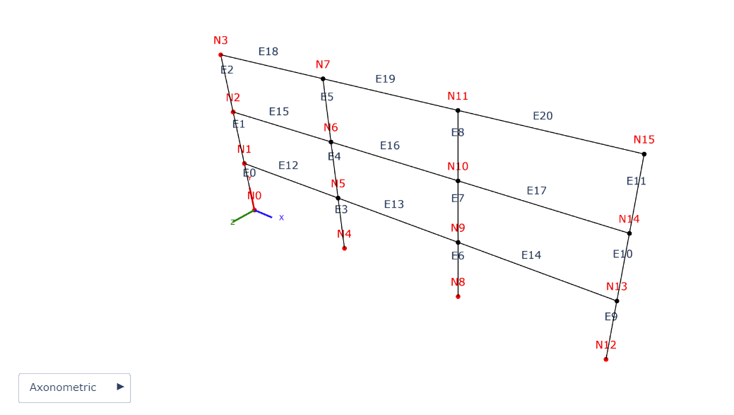
fapp.plotter.plot(structure) for visualizing geometry, node and element tags, and connectivity.
- structure: {fapp.Analysis}
- Pass in the structure you want to visualize
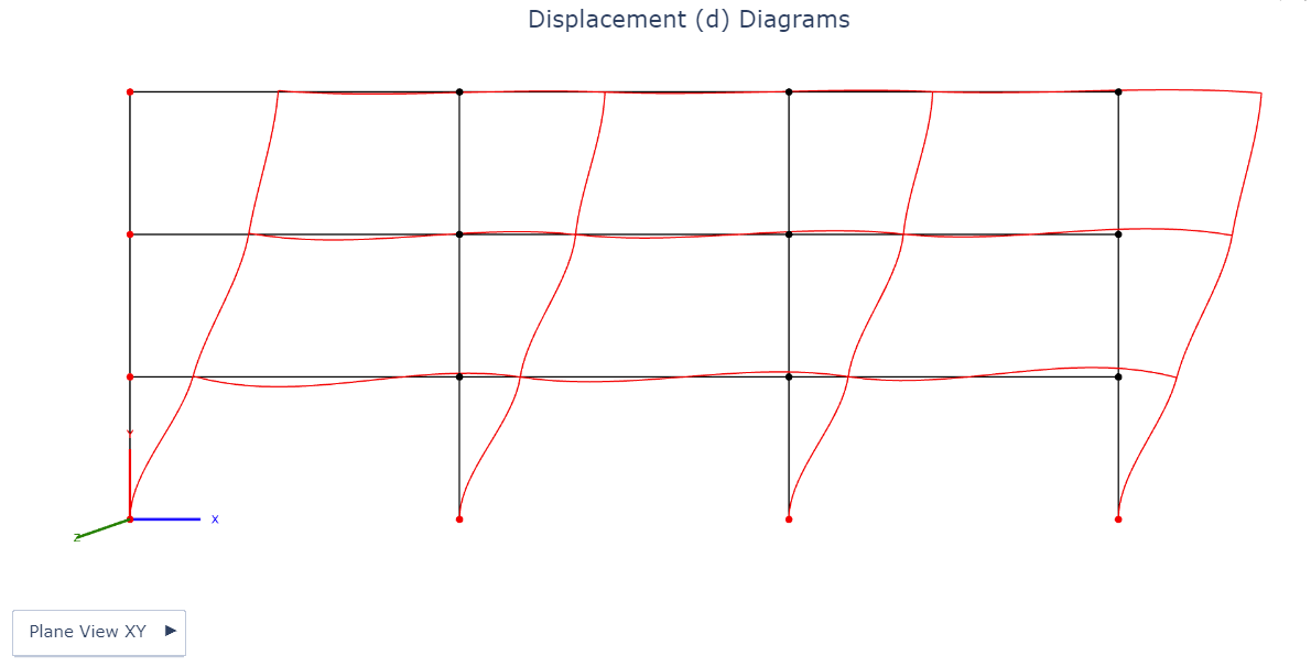
fapp.plotter.plot_results(structure, display="d", scale=15, show_value = False) for results after analysis such as displacement and force diagrams.
- structure: {fapp.Analysis}
- Pass in the structure you want to visualize
- display: string (optional)
- Indicate what result you wish to see. Default = "d"
- "d" - displacement
- "N" - axial
- "Vy" - shear in local y axis (major bending direction)
- "Vz" - shear in local z axis (minor bending direction)
- "Tx" - torsion
- "My" - moment about local y axis (minor bending direction)
- "Mz" - moment about local z axis (major bending direction)
- scale: float (optional)
- Scale of displacement or force diagram. Adjust manually as needed. 15 seems to be a good number. Larger number = larger scale. Default = 15
- show_value: boolean (optional)
- Show force diagram magnitude at the two ends. Gets quite cluttered so it is off by default. Default = False
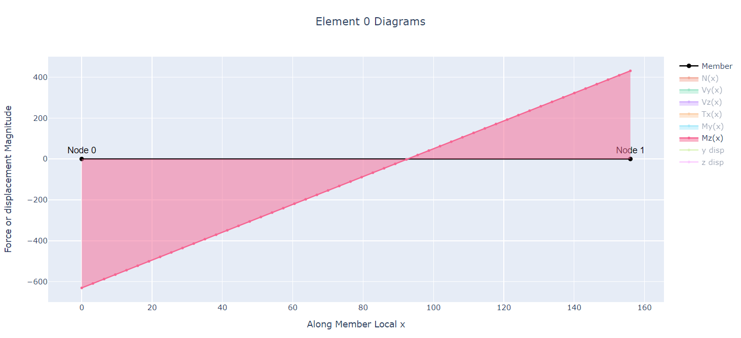
fapp.plotter.plot_diagrams(structure, ele_tag) for displacement and force diagrams for a single element about its local coordinate system.
- structure: {fapp.Analysis}
- Pass in the structure you want to visualize
- ele_tag: int
- Element tag to identify which element you would like to plot
Notes and Assumptions
- Global Coordinate (X, Y, Z):
- Y is the vertical axis (Elevation)
- X and Z are the axes within the horizontal plane (Plan)
- Recommend modeling 2-D plane structures in the X-Y plane
- Recommend modeling 2-D floor grids in the X-Z plane
- Local Coordinate (x, y, z):
- x-axis = element longitudinal axis
- z-axis = element major bending axis (relevant section properties: Iz, Ayy)
- y-axis = element minor bending axis (relevant section properties: Iy, Azz)
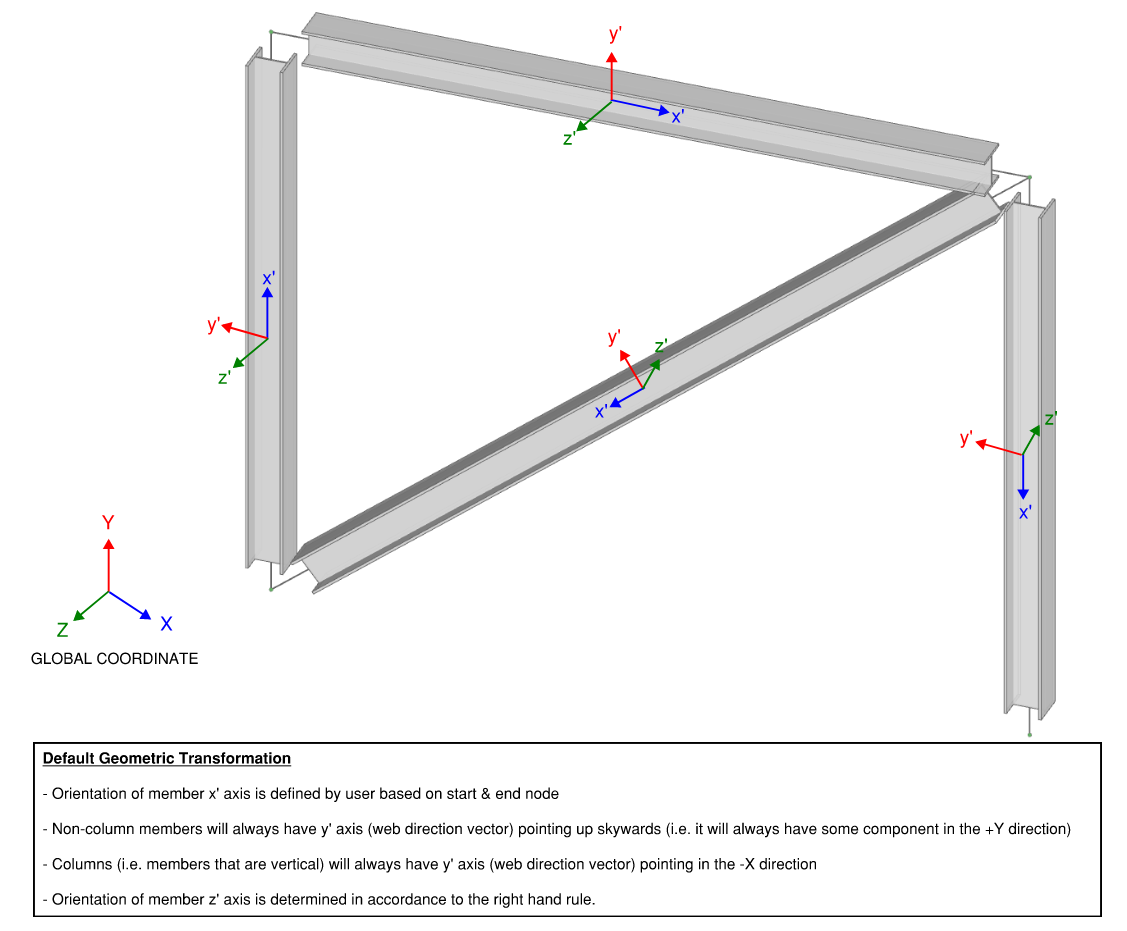
- Default geometric transformation (i.e. member orientation):
- Element major axis (web direction vector) always points skyward
- For elements that are completely vertical (columns), major axis always points towards -X
- This default setting works well because beams will always have major section properties resisting gravity load, and columns will always have major section properties when modeling within the X-Y plane
- fapp is agnostic when it comes to unit. Please ensure your input is consistent
License
MIT License
Copyright (c) 2023 Robert Wang
Release history Release notifications | RSS feed


Download files
Download the file for your platform. If you're not sure which to choose, learn more about installing packages.
Source Distribution
Built Distribution
Filter files by name, interpreter, ABI, and platform.
If you're not sure about the file name format, learn more about wheel file names.
Copy a direct link to the current filters
File details
Details for the file fapp-1.0.1.tar.gz.
File metadata
- Download URL: fapp-1.0.1.tar.gz
- Upload date:
- Size: 3.6 MB
- Tags: Source
- Uploaded using Trusted Publishing? No
- Uploaded via: twine/6.1.0 CPython/3.11.0
File hashes
| Algorithm | Hash digest | |
|---|---|---|
| SHA256 |
8ebd986dca864bc15e091c148aba92a4b5c42ad7ec126d4cfe9bff104ad5dbe8
|
|
| MD5 |
2b92de56518d0d01be50bdcacd7a6969
|
|
| BLAKE2b-256 |
be2dfd973a2c0a4a6103bb5a940edd47093982f8be27bdacd728c0064fd4900b
|
File details
Details for the file fapp-1.0.1-py3-none-any.whl.
File metadata
- Download URL: fapp-1.0.1-py3-none-any.whl
- Upload date:
- Size: 19.5 kB
- Tags: Python 3
- Uploaded using Trusted Publishing? No
- Uploaded via: twine/6.1.0 CPython/3.11.0
File hashes
| Algorithm | Hash digest | |
|---|---|---|
| SHA256 |
0b506768d3ddcae1a348402a71785160ce829186d30aeb8a64d9593fa0aabafe
|
|
| MD5 |
52c6dd5600e4006d655b73e7873e4477
|
|
| BLAKE2b-256 |
b11d6c311b26c6fb2350535b420f4b4706e5ef976daee4ac325498c3500ec2d4
|


