farofa
Failure And Repair simulation Optimization FrAmework
A Python framework for Monte Carlo simulation of repairable systems, with focus on reliability analysis. farofa enables modeling devices subject to failure and repair processes using common lifetime distributions, including imperfect repair models such as the Generalized Renewal Process (GRP).
Status: Early development (pre-release). The API is unstable and subject to change.
Features
- Single-device failure-repair simulation with configurable failure and repair time distributions
- Fleet simulation with
nidentical devices sharingkmaintenance teams (FIFO queue) - Lifetime distributions: Exponential, Weibull (perfect repair), Weibull with minimal repair, Weibull GRP (Kijima Type I and Type II), Lognormal, Normal, Gamma
- Custom user-defined distributions via callable factories
- Monte Carlo replication for statistical analysis (failures, availability, MTTF, MTTR, utilization, queue/wait metrics)
- Reproducible by construction:
simulate(seed=...)gives bit-for-bit repeatable runs (same environment), with provably independent per-device PCG64 streams vianumpy.random.SeedSequence - Vectorized random variate generation (buffered batch draws through NumPy's PCG64 generator)
- Parameter estimation from failure records: power-law NHPP (Crow-AMSAA), Weibull GRP (Kijima I/II) by maximum likelihood, and the Laplace trend test, with fits that plug straight into a simulation
- Graphical interface (
farofa gui): build a model, run it and explore the results in the browser without writing code; works offline, in Portuguese or English
Installation
pip install farofa
From a checkout of this repository:
git clone https://github.com/jmateusms/farofa.git
cd farofa
pip install -e .
Graphical interface
farofa gui # or: python -m farofa gui
This starts a small local server (Python standard library only, no extra
dependencies, no internet access needed) on http://127.0.0.1:8765/ (or the
next free port) and opens it in the browser. Options: --port N,
--no-browser, and --host (default 127.0.0.1, this machine only). Stop it
with Ctrl+C. The interface follows the browser language (Portuguese or
English) and has a PT/EN switch in the top bar.
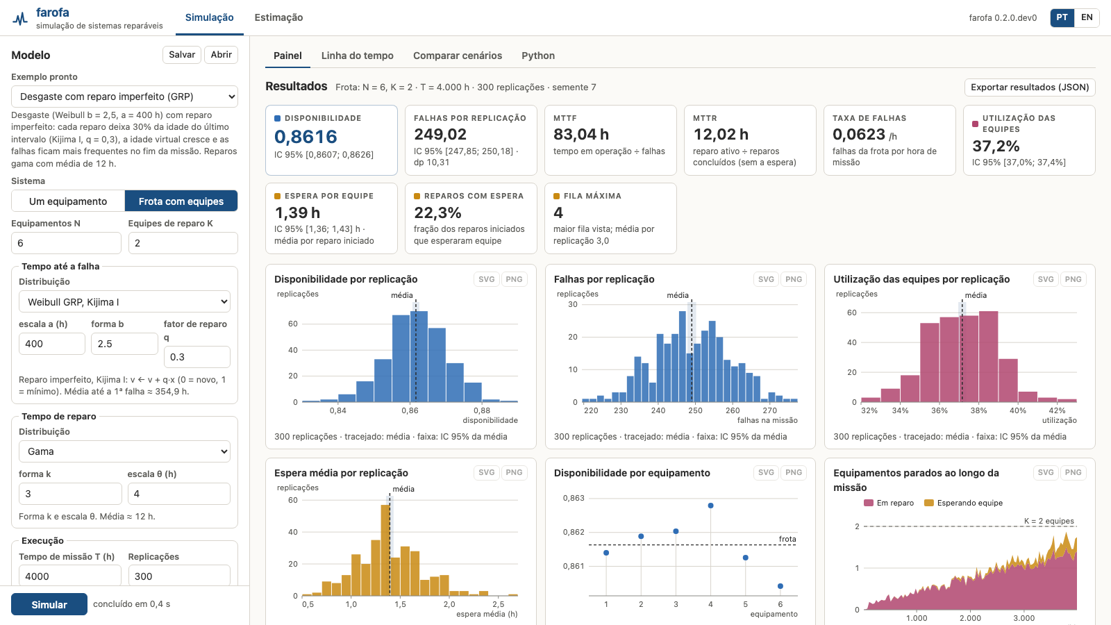
Simulation. The model panel on the left builds a single device or a fleet of N devices sharing K repair teams, with any built-in failure and repair distribution, mission time, replications, seed and number of traced replications. Fields are checked by the engine itself, so its messages appear under the offending field. Ready-made examples load a model in one click, and Save/Open keep a scenario as JSON. Long runs show progress and can be cancelled. The results tabs on the right:
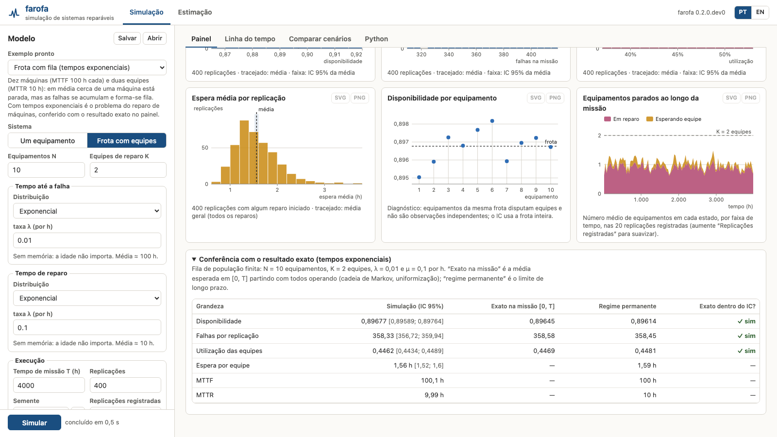
- Dashboard: availability, failures per replication, MTTF, MTTR and failure
rate; for fleets, team utilization, wait for a team, share of repairs that
waited and maximum queue. Intervals are the library's 95% intervals (one
observation per replication); the wait interval is a delta-method interval
of the pooled ratio computed by the interface. Histograms show the outcome
of every replication, a dot plot the availability of each device, and an
area chart the mean number of devices waiting or in repair over the mission
(from the traced replications). With exponential times, the run is checked
against the exact finite-source queue (Markov chain). Export results
downloads the engine's
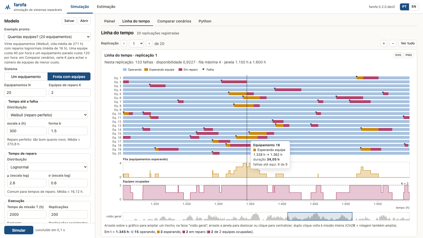
to_dict()plus the scenario. - Timeline: one traced replication as a Gantt chart (up / waiting for a team / in repair, failure markers), with queue length and busy teams below. Drag across it to zoom, pan with the overview strip, hover for details.
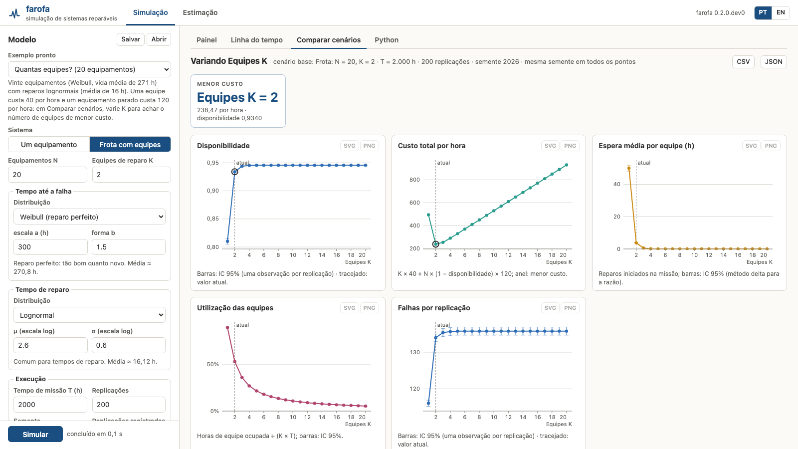
- Compare scenarios: varies one parameter (teams K, devices N, mission time or any distribution parameter such as q) with the same seed at every point, and plots availability, wait, utilization and failures against it with intervals; optional costs per team-hour and per device-hour down give the cheapest number of teams. Table as CSV or JSON.
- Python: the script that reproduces the model with farofa.
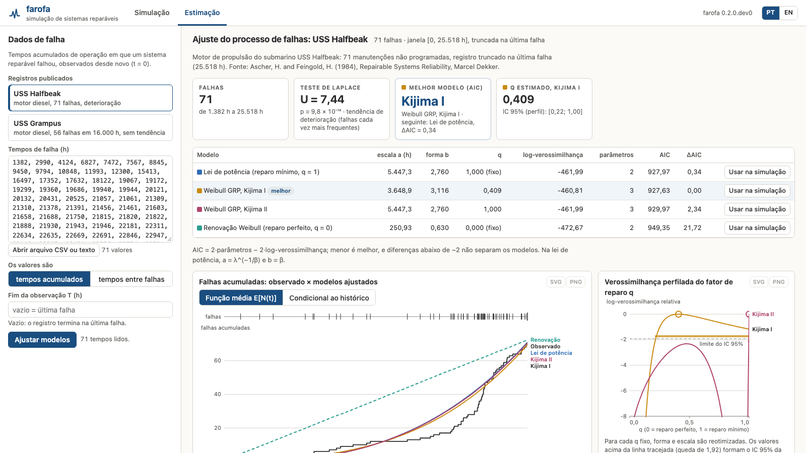
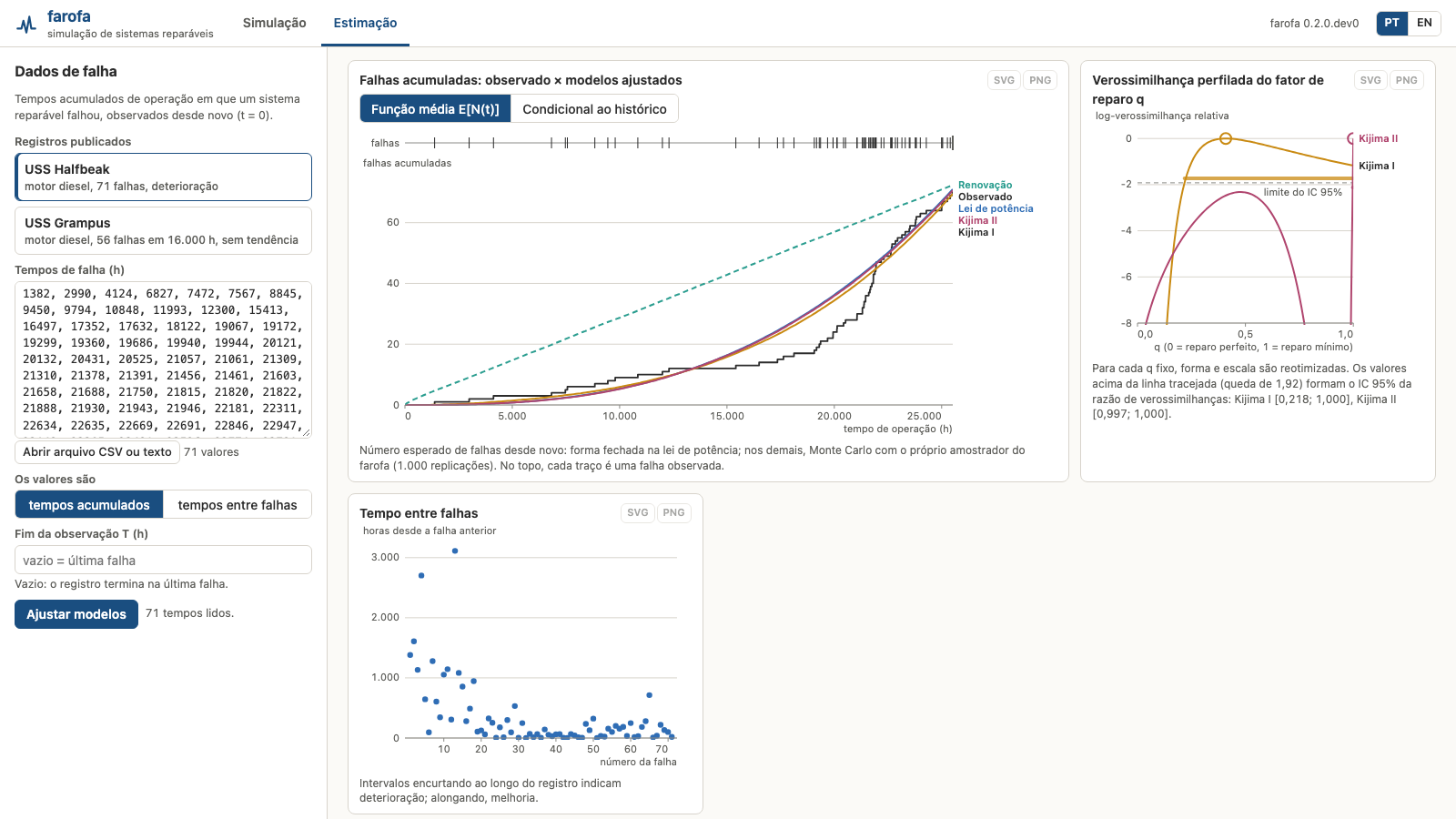
Estimation. Paste or open failure times (one system, cumulative operating hours or times between failures, optional end of observation), or load the USS Halfbeak or USS Grampus records. The view shows the Laplace trend test, the power law, Weibull GRP Kijima I and II and the Weibull renewal process with AIC, observed cumulative failures against each fitted mean function (or against the cumulative intensity given the observed history), the profile likelihood of q with 95% likelihood-ratio intervals, and the times between failures. Use in simulation sends a fit to the model panel.
Every chart can be saved as SVG or PNG. More screenshots: timeline, team sizing, exact check, Halfbeak estimation and its curves.
Quick start
Single device
import farofa

device = farofa.SimpleDevice()
device.set_failure_dist('exponential', 0.0001)  # rate = 0.0001 failures/hour
device.set_repair_dist('exponential', 0.01)      # rate = 0.01 repairs/hour
device.set_mission_time(8760)                     # 1 year in hours

result = device.simulate(reps=10000)
print(result)
Fleet with shared maintenance teams
import farofa

fleet = farofa.Fleet(n_devices=10, n_teams=2)
fleet.set_failure_dist('weibull_grp', 200.0, 1.8, 0.4)  # imperfect repair
fleet.set_repair_dist('lognormal', 2.0, 0.4)
fleet.set_mission_time(8760)

result = fleet.simulate(reps=200)
print(result)
Reproducible runs
Pass seed= to simulate() to make a run bit-for-bit reproducible (in the
same environment). Each sampler — and each device in a fleet — draws from its
own independent PCG64 stream spawned from the seed, so the random sequence a
device consumes never depends on fleet size (full trajectories are also
identical across fleet sizes when there is no repair queueing, i.e.
n_teams >= n_devices):
r1 = device.simulate(reps=10000, seed=42)
r2 = device.simulate(reps=10000, seed=42)
# r1 and r2 are identical, sample by sample
Custom distribution factories work too: a plain callable is accepted but sits
outside seed control; implement set_rng(generator) (or subclass
farofa.distributions.Sampler) to participate in seeding.
Uncertainty from replications
Availability results expose a normal-approximation confidence interval based on one outcome per replication:
result.availability_confidence_interval()  # (lower, upper), 95% by default
result.failure_count_confidence_interval() # mean total failures per replication
For a fleet, the outcome is the whole fleet's device-hour availability in a
replication, rather than one value per device: shared maintenance teams induce
within-replication dependence. The interval describes Monte Carlo sampling
error only. It does not remove the established [0, T) mission-boundary
censoring or model uncertainty; with fewer than two replications it returns
(nan, nan). Fleets also expose server_utilization_confidence_interval();
it uses busy_team_hours / (n_teams * mission_time) once per replication.
Reproducible result export and illustrative sizing
Both result types provide to_dict() and export_json(path). The export is a
versioned JSON payload with summary metrics, confidence intervals and the raw
outcome for every replication. Unavailable numerical estimates are exported as
JSON null (while the Python API retains nan). In fleet outputs, those whole-fleet replication
outcomes are the unit for intervals; per-device rows are diagnostic only.
examples/illustrative_team_sizing.py is a runnable synthetic comparison of
one, two and three maintenance teams. It records its seed, replication budget,
finite-horizon convention and all assumptions in
illustrative_team_sizing_results.json. Its values are deliberately invented
for a reproducible example and are not a real staffing recommendation.
From failure data to simulation
farofa.estimation fits a failure process to the cumulative operating times
at which one system failed, observed from new (t = 0) until end_time
(failure-truncated at the last failure when omitted):
import farofa

times = [...]  # cumulative operating hours at each failure, ascending
u, p = farofa.laplace_trend_test(times, end_time=T)  # u > 0: deterioration
nhpp = farofa.fit_power_law(times, end_time=T)        # minimal repair (q = 1)
grp = farofa.fit_weibull_grp(times, end_time=T)        # Kijima I, q estimated
print(nhpp.b, grp.q, grp.aic, nhpp.aic)

device = farofa.SimpleDevice()
device.set_failure_dist(*grp.distribution())   # ('weibull_grp', a, b, q)
device.set_repair_dist('lognormal', 2.0, 0.4)  # repair times fitted separately
The power law has a closed form. For the GRP the scale is profiled out and
the likelihood is maximized over shape and q (grid plus golden-section
search, NumPy only); fit_weibull_grp(..., q=value) fixes q, so a loop over
q traces its profile likelihood for interval estimates. q = 1 reproduces
the power law and q = 0 a Weibull renewal process. Repair durations do not
enter these likelihoods.
examples/repairable_data_fit.py runs the whole path on two published
diesel-engine records (USS Halfbeak, which deteriorates, and USS Grampus,
which shows no trend).
Event trace and timelines
simulate(..., trace=k) records the events of the first k replications — FAILURE,
REPAIR_START (a team takes the device, possibly after queueing) and REPAIR_DONE — in
result.event_log, a structured array with columns rep, entity, event, time. Recording
draws no random numbers, so every metric is identical with or without it.
result = fleet.simulate(reps=1000, seed=42, trace=3)
result.event_log[:5]            # (rep, device, event, time) rows
tl = result.timeline(0)         # (entity, state, start, end); state: up / waiting / repair
Counting waiting and repair intervals over time gives the queue length and the busy
teams; to_dict() / export_json() include the event log when a trace was recorded.
simulate(..., progress=f) calls f(done, reps) after every replication (the GUI uses it
for its progress bar and to cancel a run by raising from f); like the trace, it draws no
random numbers and changes no result.
Available distributions
| Distribution | Function | Repair assumption | Parameters |
|---|---|---|---|
| Exponential | exponential |
Memoryless (perfect repair) | rate |
| Weibull | weibull |
Perfect repair (age reset to 0) | a (scale), b (shape) |
| Weibull (minimal repair) | weibull_min |
Minimal repair (age preserved; stateful) | a (scale), b (shape) |
| Weibull GRP (Kijima I) | weibull_grp |
Imperfect repair, v_i = v_{i-1} + q·x_i (stateful) |
a (scale), b (shape), q (repair effectiveness, 0–1) |
| Weibull GRP (Kijima II) | weibull_grp2 |
Imperfect repair, v_i = q·(v_{i-1} + x_i) (stateful) |
a (scale), b (shape), q (repair effectiveness, 0–1) |
| Lognormal | lognormal |
— (typically used for repair times) | mu, sigma (log-scale) |
| Normal (truncated at 0) | normal |
— (resampled until positive) | mu, sigma |
| Gamma | gamma |
— | shape, scale |
Roadmap
farofa is being developed incrementally. Below is the planned scope for each milestone. The versioned current-state plan is docs/DEVELOPMENT_PLAN.md.
v0 — Single device simulation
Core simulation engine for a single repairable device.
- Failure-repair simulation loop with exponential and Weibull distributions
- Weibull GRP (Generalized Renewal Process) for imperfect repair modeling (Kijima Type I and Type II)
- Reproducible, vectorized random variate generation (PCG64, seeded per-device streams)
- Support for custom (user-defined) lifetime distributions
- Lognormal, Normal, and Gamma distributions
- Output metrics: availability, mean time to failure (MTTF), mean time to repair (MTTR), failure rate
- Results object with summary statistics and raw simulation data
- Input validation and meaningful error messages
- Unit tests
- CI: pytest on supported Python versions
v1 — Queueing systems (current)
Multiple devices sharing repair resources (maintenance teams).
- Queue with
nidentical devices andkrepair servers (FIFO) - Metrics: queue length, waiting time, server utilization
- Additional queue disciplines (priority-based, custom)
- Support for custom queue models
v2 — Heterogeneous systems
Different device types in the same system.
- Multiple device types with independent failure/repair behavior
- Priority classes for repair scheduling
- System-level metrics (e.g., system availability with redundancy)
- Expanded set of output metrics
v3 — Optimization
Find optimal maintenance policies and system configurations.
- Optimization over maintenance parameters (e.g., preventive maintenance interval, number of repair teams)
- Built-in objective functions: cost, availability, profit
- Support for custom objective functions
- Integration with scipy.optimize or similar
v4 — GUI
Graphical interface for building and running simulations without code.
- Local web interface (
farofa gui, standard library only, offline): model builder validated by the engine, scenario files, progress and cancel - Results dashboard with confidence intervals, per-replication histograms, interactive timeline (zoom, hover), queue and busy teams over time, SVG/PNG/JSON export
- Scenario comparison (one-parameter sweeps with common random numbers, cost-based team sizing)
- Estimation view: Laplace test, power-law and GRP fits with AIC, mean functions, profile likelihood of q, fit sent to the simulation
- Portuguese and English
- Views for heterogeneous systems and optimization (following v2 and v3)
v5 — Parameter estimation
Estimate distribution parameters from observed failure/repair data.
- Maximum likelihood estimation for repairable-system failure processes (power-law NHPP, Weibull GRP Kijima I/II) and the Laplace trend test
- Maximum likelihood estimation for the remaining (repair-time) distributions
- Goodness-of-fit testing
- Integration with or reference to existing tools (e.g.,
reliabilitypackage)
Background
farofa is inspired by research in reliability engineering, particularly repairable systems modeling with imperfect repair and queueing-based maintenance optimization. Key references:
- Moura, M. C. et al. (2017). Analysis of extended warranties for medical equipment: A Stackelberg game model using priority queues. Reliability Engineering & System Safety, 168, 338–354. DOI
- Santana, J. M. et al. (2018). Extended warranty of medical equipment subject to imperfect repairs. Eksploatacja I Niezawodnosc, 20(4), 567–578. DOI
- Yañez, M. et al. (2002). Generalized renewal process for analysis of repairable systems with limited failure experience. Reliability Engineering and System Safety, 77(2), 167–180. DOI
- Wang, Z. M. & Yang, J. G. (2012). Numerical method for Weibull generalized renewal process and its applications in reliability analysis of NC machine tools. Computers and Industrial Engineering. DOI
- Moura, M. C. et al. (2014). A competing risk model for dependent and imperfect condition-based preventive and corrective maintenances. Proceedings of the Institution of Mechanical Engineers Part O, 228(6), 590–605. DOI
Citing
If you use farofa in academic work, please cite it: GitHub's Cite this repository button (from CITATION.cff) gives APA and BibTeX.
License
BSD 3-Clause — see LICENSE. Versions up to 0.2.0 were released under the GNU General Public License v3.
1 maintainer

Metadata
1 maintainer
Release files for farofa 0.2.1
For a detailed explanation of source distributions (sdists) and built distributions (wheels), please see the package formats documentation.
Source distribution (sdist)
| File | Size | Uploaded | |
|---|---|---|---|
| farofa-0.2.1.tar.gz | 127.8 kB | Details |
Built distribution (wheel)
| File | Interpreter | ABI | Platform | Reset |
|---|---|---|---|---|
| farofa-0.2.1-py3-none-any.whl | Python 3 | none | any | Details |
Total release size: 234.7 kB
Release files / farofa-0.2.1.tar.gz
| Download URL | farofa-0.2.1.tar.gz |
|---|---|
| Size | 127.8 kB |
| Tags | Source |
|
SHA-256 checksum How to use checksums |
87ed44a9317e7e3278f12c62693cf29bca16711e543ab170b244ed002d0581df
|
|
BLAKE2b-256 checksum How to use checksums |
25a67162cf91d2d899b94f978ebb2f57c14242d3d1894fef11c6b31c5bc7f66a
|
| Upload date | |
|
Uploaded using Trusted Publishing? What is trusted publishing? |
No |
| Uploaded via |
twine/7.0.0 CPython/3.12.12
|
Release files / farofa-0.2.1-py3-none-any.whl
| Download URL | farofa-0.2.1-py3-none-any.whl |
|---|---|
| Size | 106.9 kB |
| Tags | Python 3 |
|
SHA-256 checksum How to use checksums |
9e236a63af5a9175893e53c96983bf406f6bd2369fbf401e8eb1a1a6e8d4e3ac
|
|
BLAKE2b-256 checksum How to use checksums |
619d91d69eed5b24b99b58ea7ce5ab3532a0c1f2fb444ee9d5c6259240a15ab8
|
| Upload date | |
|
Uploaded using Trusted Publishing? What is trusted publishing? |
No |
| Uploaded via |
twine/7.0.0 CPython/3.12.12
|