
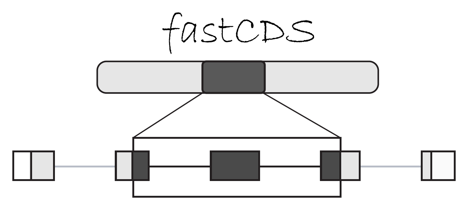
Fast, exact protein-to-genome coordinate mapping
map a protein feature's amino-acid range onto its genomic exon and CDS structure





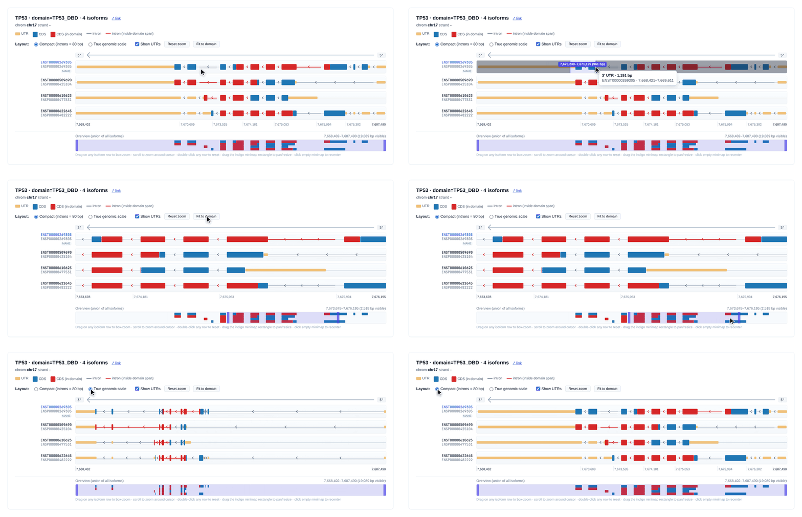
The TP53 DNA-binding domain mapped across four isoforms on a shared genomic axis (self-contained interactive viewer).
Map protein-domain amino-acid coordinates to their underlying genomic CDS / UTR / intron structure, using any Ensembl, GENCODE, or NCBI RefSeq GTF.
For each input query (a protein_id or a transcript_id, optionally with an aa range), fastCDS answers two related but distinct questions:
- Mapping - which exact genomic bases code this domain?
- Structure - how is the whole transcript organised in 5'UTR / CDS / 3'UTR / intron, and where does the domain fall on it?
A C++17 binary does the heavy lifting: once the index is loaded, the mapping itself is ~1 us per query, so end-to-end throughput is dominated by output formatting (~5,800 queries/s for a single-isoform TSV, ~2,800 q/s writing the full --output all set). fastCDS produces three kinds of output: a BED12 track for genome browsers, a static figure (matplotlib PDF/PNG/SVG), and an interactive HTML viewer. A Python wrapper adds pandas DataFrames; for the viewer you pick the engine (self-contained vanilla JS by default, or plotly).
📖 Full documentation lives in the wiki
Install
pip install fastCDS                                 # pre-built wheel: binary + wrapper (Linux/macOS)
mamba install -c bioconda -c conda-forge fastCDS    # or via conda/mamba
pixi add -c bioconda -c conda-forge fastCDS         # or via pixi
The pip wheel bundles the compiled binary, so all four commands work immediately. On platforms without a wheel (e.g. Windows) pip builds from source - see Installation for the toolchain and a from-source build.
Quickstart
The workflow is three steps - get an index (index from a GTF, or fetch a pre-built one), map your domain queries onto it, then plot:
flowchart TB
    GTF[GTF annotation] --> INDEX([fastCDS index])
    ZEN[Zenodo] --> FETCH([fastCDS fetch])
    INDEX --> IDX[index<br/>human.idx]
    FETCH --> IDX
    BED[query BED<br/>protein + aa range] --> MAP([fastCDS map])
    IDX --> MAP
    MAP --> TSV[isoform_structure.tsv]
    MAP --> BEDS[BED tracks<br/>bed12 + coding<br/>introns / span]
    MAP --> TAB[feature + summary TSVs<br/>coding / introns<br/>mapping_summary]
    TSV --> PLOT([fastCDS plot])
    PLOT --> STATIC[static figure<br/>.pdf / .png / .svg]
    PLOT --> INTER[interactive viewer<br/>.html: js or plotly]
    BEDS --> IGV[genome browser<br/>IGV / UCSC]
    TAB --> AN[your analysis<br/>pandas / stats]

    classDef cmd fill:#2f6db0,color:#ffffff,stroke:#1c4a7d,stroke-width:1px;
    classDef file fill:#eef2ff,color:#111111,stroke:#9aa7d0,stroke-width:1px;
    class INDEX,FETCH,MAP,PLOT cmd;
    class GTF,ZEN,IDX,BED,TSV,BEDS,TAB,STATIC,INTER,IGV,AN file;
# 1. Get an index (one-time per annotation)
fastCDS index --gtf my.gtf --out human.idx   # build from a GTF you already have
# or skip the GTF - grab a pre-built index from Zenodo:
fastCDS fetch human --out human.idx

# 2. Map a BED of domain queries
fastCDS map \
    --index human.idx \
    --bed queries.bed --out-dir results --output all --threads 8

# 3. Plot a single domain - the --out extension picks the format
fastCDS plot \
    --isoform results/isoform_structure.tsv \
    --input-id TP53_DBD \
    --out tp53_dbd.pdf              # static figure (.pdf/.png/.svg)
#   --out tp53_dbd.html            # interactive viewer (vanilla JS by default)
#   --out tp53_dbd.html --engine plotly
Run fastCDS fetch list to see every target and source.
The same workflow from Python:
import fastCDS as fc

# 1. Get an index (one-time)
idx = fc.build_index("my.gtf", out="human.idx")    # build from a GTF; Path-returning
# idx = fc.fetch_index("human")                    # or grab a pre-built one from Zenodo

# 2. Map queries
mapper = fc.Mapper(index=str(idx))
result = mapper.map_batch([
    {"protein_id": "ENSP00000269305", "aa_start": 102, "aa_end": 292, "domain_id": "TP53_DBD"},
])
result.summary       # one-row DataFrame
result.isoform       # plot-ready DataFrame

# 3. Plot - the out extension picks the format; engine picks the HTML renderer
fc.plot(result, input_id="TP53_DBD", out="tp53_dbd.pdf")                    # static figure
fc.plot(result, input_id="TP53_DBD", out="tp53_dbd.html")                   # interactive (vanilla JS)
fc.plot(result, input_id="TP53_DBD", out="tp53_dbd.html", engine="plotly")  # interactive (plotly)
Full reference: Building an index, Mapping, Plotting, Python API.
Validation + benchmarks
- 100.00 % exact match vs ensembldb on 5,000 stratified queries (9 strata covering single/multi-exon, both strands, codon-split, selenoproteins, incomplete CDS) - zero off-by-ones, zero structural mismatches.
- ~980x faster than ensembldb (also ~4,560x Ensembl REST) - measured end-to-end: total wall time from process start to all results written, including the one-time index load, over N = 10,000 queries on one thread (fastCDS 5,886 q/s vs ensembldb 6.0 q/s; REST at N = 1,000, the largest it finishes). The gap grows with N because fastCDS amortizes its ~1.5 s index load; the per-query mapping itself, once loaded, is faster still.
- Full design, numbers, and scaling curves: Performance and benchmarking. Reproduce via
reproduce_benchmarking_figures/benchmarks/README.md.
Notebooks
Worked examples under tutorial/ - each opens in Colab or nbviewer. They reproduce the manuscript's example analyses; see reproduce_benchmarking_figures/README.md and reproduce_isoform_figures/README.md for run order.
| Notebook | What it covers |
|---|---|
walkthrough_end_to_end.ipynb (view on nbviewer) |
Zero-to-figure tour: fetch_index -> BED prep -> map_batch -> all plot styles. The interactive HTML viewers only render on nbviewer, not GitHub. |
reproduce_isoform_figures/ |
Projects every source-isoform Pfam domain onto a gene's alternative isoforms and scores retention (intact / skipped / trimmed) - the analysis behind Figure 1C-F. |
software_comparison.ipynb |
Accuracy + speed: per-category agreement vs ensembldb / GenomicFeatures / TransVar / Ensembl REST (Table S1), and throughput + RSS vs ensembldb / GenomicFeatures / geneplot / REST (Table S2), on the same human set. |
scaling_and_ram.ipynb |
fastCDS measured against itself (not other tools): wall-clock + peak-RSS scaling curves, OpenMP speedup, and the --batch-size RAM cap at N = 1 M. |
Citation
A formal citation will land when the accompanying manuscript is posted. Until then, please cite the repository URL: https://github.com/SotoLF/fastCDS. See also CITATION.cff.
License
MIT - see LICENSE.
Maintainers
- Owner: Luis F. Soto Ugaldi (@SotoLF)
- Collaborator: George D. Muñoz Esquivel (@george123ya)
Issues and pull requests welcome.
1 maintainer

Download files
Download the file for your platform. If you're not sure which to choose, learn more about installing packages.
Source Distribution
File details
Details for the file fastcds-2.3.0.tar.gz.
File metadata
- Download URL: fastcds-2.3.0.tar.gz
- Upload date:
- Size: 2.1 MB
- Tags: Source
- Uploaded using Trusted Publishing? No
- Uploaded via: twine/6.2.0 CPython/3.11.15
File hashes
| Algorithm | Hash digest | |
|---|---|---|
| SHA256 |
cee176dd7b45e5749c955e1cc44bee6d7eb5778b905eed98248c672e51fda3e0
|
|
| MD5 |
6ac0b8ce523303242326a49e35474135
|
|
| BLAKE2b-256 |
11191a7e58a5edd3b0b5e9f7c52dc58c3443797867572c56dc4dba6d6a7e306b
|







