
FastBootstrap
⚡ Fast Python implementation of statistical bootstrap methods




High-performance statistical bootstrap with parallel processing and comprehensive method support
Installation • Quick Start • Examples • Performance • API
🚀 Features
- Multiple Bootstrap Methods: Percentile, BCa, Basic, Studentized, Spotify-style, and Poisson bootstrap
- High Performance: Parallel processing with joblib, optimized NumPy operations
- Smart Batch Sizing: Intelligent auto-optimization, up to 30% faster than naive batch sizes with zero tuning
- Comprehensive Statistics: Confidence intervals, p-values, effect sizes, power analysis, quantile-quantile analysis
- Flexible API: Unified interface with method auto-selection
- Rich Visualizations: Built-in plotting with matplotlib and plotly
- Production Ready: Extensive error handling, type hints
📦 Installation
pip install fastbootstrap
To also pull Jupyter for running the example notebook locally:
pip install "fastbootstrap[notebook]"
🛠️ Development Setup
Install uv: https://docs.astral.sh/uv/getting-started/installation/
git clone https://github.com/timofeytkachenko/fastbootstrap.git
cd fastbootstrap
uv sync
source .venv/bin/activate
pre-commit install
🎯 Quick Start
import numpy as np
import fastbootstrap as fb

# Generate sample data
np.random.seed(42)
control = np.random.normal(100, 15, 1000)      # Control group
treatment = np.random.normal(105, 15, 1000)    # Treatment group (+5% effect)

# Two-sample bootstrap test with smart batch sizing
result = fb.two_sample_bootstrap(
    control, treatment,
    batch_size='smart',  # Auto-optimize performance ✨
    plot=True
)
print(f"P-value: {result['p_value']:.4f}")
print(f"Effect size: {result['statistic_value']:.2f}")
print(f"95% CI: [{result['confidence_interval'][0]:.2f}, {result['confidence_interval'][1]:.2f}]")
📊 Examples
One-Sample Bootstrap
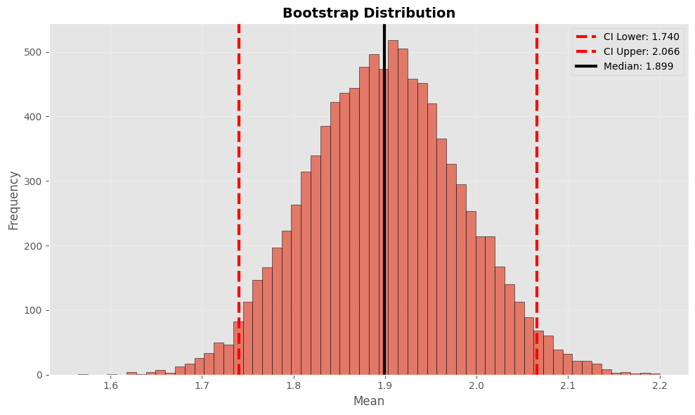
Estimate confidence intervals for a single sample statistic:
import fastbootstrap as fb
import numpy as np

# Sample data
sample = np.random.exponential(2, 500)

# Basic percentile bootstrap
result = fb.one_sample_bootstrap(
    sample,
    statistic=np.mean,
    method='percentile',
    bootstrap_conf_level=0.95,
    number_of_bootstrap_samples=10000,
    plot=True
)

print(f"Mean estimate: {result['statistic_value']:.3f}")
print(f"95% CI: [{result['confidence_interval'][0]:.3f}, {result['confidence_interval'][1]:.3f}]")

# Advanced: BCa (Bias-Corrected and Accelerated) bootstrap
bca_result = fb.one_sample_bootstrap(
    sample,
    method='bca',
    statistic=np.median,
    plot=True
)
Two-Sample Comparison
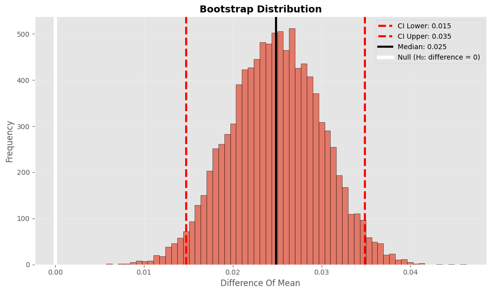
Compare two groups with various statistics:
import fastbootstrap as fb
import numpy as np

# A/B test data
control = np.random.normal(0.25, 0.1, 800)     # 25% conversion rate
treatment = np.random.normal(0.28, 0.1, 800)   # 28% conversion rate

# Test difference in means
result = fb.two_sample_bootstrap(
    control,
    treatment,
    statistic=fb.difference_of_mean,
    number_of_bootstrap_samples=10000,
    plot=True
)

print(f"Difference in conversion rates: {result['statistic_value']:.1%}")
print(f"P-value: {result['p_value']:.4f}")
print(f"Significant: {'Yes' if result['p_value'] < 0.05 else 'No'}")

# Test percentage change
percent_result = fb.two_sample_bootstrap(
    control,
    treatment,
    statistic=fb.percent_change_of_mean
)
print(f"Percentage change: {percent_result['statistic_value']:.1%}")
Spotify-Style Bootstrap
Fast quantile-based bootstrap using binomial sampling:
import fastbootstrap as fb
import numpy as np

# Revenue data (heavy-tailed distribution)
control_revenue = np.random.lognormal(3, 1, 1000)
treatment_revenue = np.random.lognormal(3.1, 1, 1000)

# Compare medians (50th percentile)
result = fb.spotify_two_sample_bootstrap(
    control_revenue,
    treatment_revenue,
    q1=0.5,  # Median
    q2=0.5,
    plot=True
)

print(f"Median difference: ${result['statistic_value']:.2f}")
print(f"P-value: {result['p_value']:.4f}")

# Compare different quantiles
p90_result = fb.spotify_two_sample_bootstrap(
    control_revenue,
    treatment_revenue,
    q1=0.9,  # 90th percentile
    q2=0.9
)
print(f"90th percentile difference: ${p90_result['statistic_value']:.2f}")
Power Analysis & Simulation
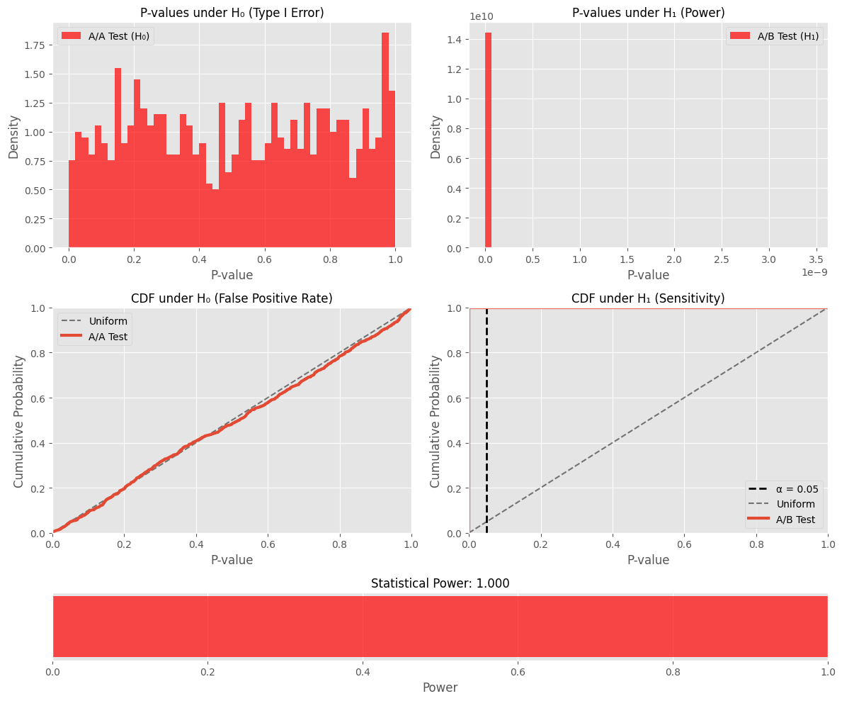
Comprehensive statistical power analysis:
import numpy as np
import fastbootstrap as fb

# Simulate experiment data
control = np.random.normal(100, 20, 500)
treatment = np.random.normal(110, 20, 500)  # 10% effect size

# Power analysis
power_result = fb.power_analysis(
    control,
    treatment,
    number_of_experiments=1000,
    plot=True
)

print("Power Analysis Results:")
print(f"Statistical Power: {power_result['power_summary']['statistical_power']:.3f}")
print(f"Type I Error Rate: {power_result['power_summary']['type_i_error_rate']:.3f}")
print(f"Effect Size: {power_result['power_summary']['treatment_mean'] - power_result['power_summary']['control_mean']:.1f}")

# A/A test validation (should show ~5% false positive rate)
aa_result = fb.aa_test_simulation(
    np.concatenate([control, treatment]),
    number_of_experiments=2000
)
print(f"A/A Test False Positive Rate: {aa_result['type_i_error_rate']:.3f}")
Quantile-Quantile Analysis
import numpy as np
import fastbootstrap as fb

# Simulate experiment data
control = np.random.exponential(scale=1 / 0.001, size=n)
treatment = np.random.exponential(scale=1 / 0.00101, size=n)

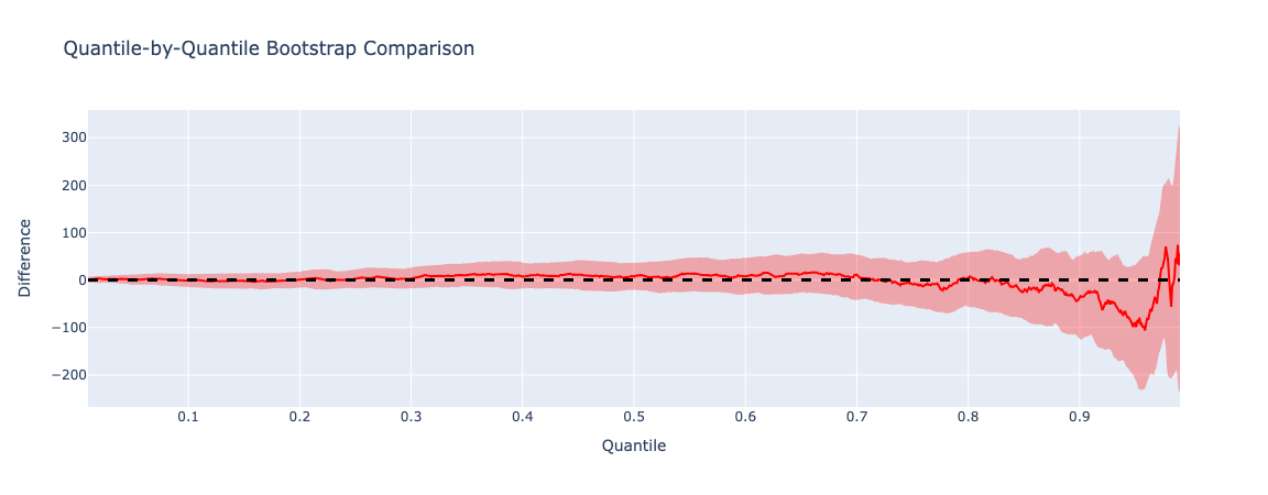
# Quantile-quantile bootstrap analysis
fb.quantile_bootstrap_plot(control, treatment, n_step=1000)
Large-Scale Bootstrap (>1M Samples)
For datasets with over 1 million bootstrap samples, use optimized batch processing:
import numpy as np
import fastbootstrap as fb

# Generate large dataset
np.random.seed(42)
large_control = np.random.lognormal(5, 1.5, 50000)
large_treatment = np.random.lognormal(5.1, 1.5, 50000)

# High-performance bootstrap with 1M samples
result = fb.two_sample_bootstrap(
    large_control,
    large_treatment,
    number_of_bootstrap_samples=1_000_000,
    n_jobs=-1,           # All CPU cores
    batch_size='smart',  # Intelligent auto-optimization (recommended)
    statistic=fb.difference_of_median
)

print(f"Median difference: {result['statistic_value']:.3f}")
print(f"P-value: {result['p_value']:.6f}")
print(f"95% CI: [{result['confidence_interval'][0]:.3f}, {result['confidence_interval'][1]:.3f}]")
Optimization Benefits:
- ~120 K bootstrap samples/s at 1M iterations on a 16-core M4 Max (see Performance)
- Peak memory is independent of
batch_size; smart mode warns before an OOM-pronen_jobs × sample_sizecombination - Suitable for production workloads with massive resampling needs
Custom Statistics
Bootstrap with simple custom statistical functions:
import numpy as np
import fastbootstrap as fb

# Simple custom statistics
def max_difference(x, y):
    """Difference in maximum values."""
    return np.max(y) - np.max(x)

def range_ratio(x, y):
    """Ratio of ranges."""
    range_x = np.max(x) - np.min(x)
    range_y = np.max(y) - np.min(y)
    return range_y / range_x

def mean_ratio(x, y):
    """Ratio of means."""
    return np.mean(y) / np.mean(x)

# Apply custom statistics
control = np.random.normal(50, 10, 300)
treatment = np.random.normal(55, 12, 300)

# Test different custom statistics
max_result = fb.two_sample_bootstrap(control, treatment, statistic=max_difference)
range_result = fb.two_sample_bootstrap(control, treatment, statistic=range_ratio)
ratio_result = fb.two_sample_bootstrap(control, treatment, statistic=mean_ratio)

print(f"Max Difference: {max_result['statistic_value']:.2f}")
print(f"Range Ratio: {range_result['statistic_value']:.3f}")
print(f"Mean Ratio: {ratio_result['statistic_value']:.3f}")
Unified Bootstrap Interface
Automatic method selection based on input:
import numpy as np
import fastbootstrap as fb

# One-sample (automatic detection)
sample = np.random.gamma(2, 2, 400)
result = fb.bootstrap(sample, statistic=np.mean, method='bca')

# Two-sample (automatic detection)
control = np.random.normal(0, 1, 300)
treatment = np.random.normal(0.3, 1, 300)
result = fb.bootstrap(control, treatment)

# Spotify-style (automatic detection)
result = fb.bootstrap(control, treatment, spotify_style=True, q=0.5)
⚡ Performance Benchmarks
Benchmarks on Apple Silicon M4 Max (16 cores, 48 GB RAM), Python 3.12.11, NumPy 2.4.4, joblib 1.5.3, fastbootstrap 1.8.6. The batch-size heuristic is unchanged in 1.8.7 and 1.8.8, so these numbers still apply.
Methodology. Each cell reports min of 3 warm runs after a 1-iteration warmup. The first joblib call pays a one-shot ~1 s loky worker-spawn penalty that is excluded by the warmup. Run-to-run noise is roughly ±3–5%, so differences below that are not significant. Reproduce by running the snippets at the end of this section.
Standard Configuration (n=1,000, bootstrap=10,000)
All methods tested with 1,000 sample size and 10,000 bootstrap iterations, library defaults (n_jobs=-1, batch_size=None).
| Method | Time (s) | Throughput (samples/s) | Performance Tier |
|---|---|---|---|
| Spotify One Sample | 0.0003 | 31,800,000 | ⚡ Ultra-fast |
| Spotify Two Sample | 0.0006 | 16,100,000 | ⚡ Ultra-fast |
| One Sample Basic | 0.138 | 72,600 | 🚀 Fast |
| Two Sample Standard | 0.139 | 71,800 | 🚀 Fast |
| One Sample Percentile | 0.141 | 70,800 | 🚀 Fast |
| One Sample BCa | 0.149 | 67,200 | 🚀 Fast |
| One Sample Studentized | 0.155 | 64,400 | 🚀 Fast |
| Poisson Bootstrap | 0.208 | 48,000 | ✓ Standard |
Performance Analysis
Method Selection Guide:
- Spotify methods: Ideal for quantile-based analysis (medians, percentiles) - 200–450x faster than standard methods
- Standard bootstrap: Best for general statistics (means, confidence intervals) - processes ~70K samples/sec
- BCa bootstrap: Advanced method with bias correction - ~5% overhead vs. percentile method (jackknife acceleration term)
- Poisson bootstrap: Specialized for aggregated comparisons - moderate performance (single-process NumPy loop)
Key Performance Insights
- Ultra-Fast Quantile Analysis: Spotify methods leverage binomial sampling for 30M+ samples/sec throughput
- Parallel Processing: Automatically distributes work across all CPU cores with optimized batch sizing
- Memory Efficient: O(n) space complexity with lazy RNG generation eliminates memory overhead
- Vectorized Operations: NumPy-optimized computations maximize throughput on modern hardware
- Linear Scalability: Performance scales linearly with sample size and bootstrap iterations
- Hardware Optimization: Process-based parallelism avoids Python GIL for true multi-core utilization
Performance Optimization with Batch Processing
The library supports intelligent batch processing for optimal performance across all dataset sizes.
Understanding batch_size
The batch_size parameter controls how many bootstrap iterations joblib dispatches to a worker per task:
- Small batches: Fine-grained load balancing, higher dispatch/IPC overhead
- Large batches: Amortised dispatch overhead, risk of idle workers on the tail of the workload
- Optimal batches: Balance dispatch overhead against load balancing for the given
Nand worker count
Peak memory is not a function of batch_size (see Peak-memory check below).
import fastbootstrap as fb
import numpy as np

# Smart mode (recommended) - automatically optimizes based on workload
result = fb.two_sample_bootstrap(
    control,
    treatment,
    number_of_bootstrap_samples=1_000_000,
    batch_size='smart'  # Intelligent batch sizing ✨ NEW
)

# Auto mode - uses joblib's default heuristics
result = fb.two_sample_bootstrap(control, treatment)

# Manual mode - explicit control for advanced users
result = fb.two_sample_bootstrap(
    control,
    treatment,
    number_of_bootstrap_samples=1_000_000,
    n_jobs=-1,          # Use all CPU cores
    batch_size=1000     # Process 1000 samples per batch
)
Smart Batch Sizing (Recommended)
The 'smart' mode automatically selects an optimal joblib batch_size from
four signals at once:
- Workload scale — number of bootstrap iterations (
number_of_bootstrap_samples). - Sample complexity — width of each resample (
sample_size_hint). - System resources — free RAM (via
psutil) and the worker count joblib will actually use (joblib.effective_n_jobs). - Load balancing — guarantees at least
MIN_BATCHES_PER_WORKER = 4chunks per worker so no core sits idle on the tail of the workload.
Smart Mode Heuristics (workload-scale base):
Bootstrap Samples (N) |
Base Batch Size | Rationale (see Batch-Size Sweep) |
|---|---|---|
N ≤ 10K |
256 | Optimum is flat 156–512; load-balancing cap binds on ≥ 16 workers |
10K < N ≤ 100K |
512 | Compromise: 16-worker optimum ≈ 1000–2000, 4-worker optimum ≈ 128–512 |
100K < N ≤ 500K |
1000 | Measured optimum on 16 workers (2000 within noise) |
N > 500K |
1000 | Measured optimum on 16 workers; ≥ 4000 is 2–4% slower |
The base value above is then narrowed by these guard rails:
- Low-RAM tier (
< MEMORY_LOW_THRESHOLD = 4 GB): cap atLOW_MEM_BATCH_CAP = 64. - Moderate-RAM tier (
4 – 8 GB): cap atBATCH_SIZE_MEDIUM = 512. Both tiers use free RAM as a proxy for "small host" and pick finer dispatch units there; they do not lower peak memory (see Peak-memory check). - Wide samples (
sample_size > LARGE_SAMPLE_THRESHOLD = 100K): divide base bySAMPLE_COMPLEXITY_DIVISOR = 2, withMIN_BATCH_FLOOR = 16as the floor. - Load-balancing cap:
max_batch = max(MIN_BATCH_FLOOR, ⌊N / (n_workers · MIN_BATCHES_PER_WORKER)⌋)— guarantees enough chunks to keep all workers busy on the tail of the workload.
Final value: clip(base, MIN_BATCH_FLOOR, max_batch).
The base lookup is a bisect_left over the public BATCH_SIZE_EDGES /
BATCH_SIZE_BASES tables (inclusive right edges), so the whole computation
is O(1) and free of branching on N.
Peak-memory check (1.8.5; replaces the per-batch memory cap of earlier releases): peak
resampling RAM is batch-invariant — each joblib worker executes its batch
sequentially and holds roughly one resample at a time, so shrinking the batch
cannot reduce the peak. Smart mode estimates the peak as
n_workers · sample_size · (dtype_bytes + INDEX_BYTES) (the + 8 accounts
for the transient int64 index array created by Generator.choice) and emits
a ResourceWarning when it exceeds MEM_FRACTION = 0.25 of available RAM,
advising to reduce n_jobs or sample_size instead of silently fragmenting
the workload into tiny batches.
CPU-core selection delegates to joblib.effective_n_jobs, so the estimate
matches the worker count Parallel actually spawns (-1 → all logical cores,
-2 → all but one, ≥ 1 → explicit count, oversubscription allowed).
Performance Benefits (measured on the same M4 Max):
- 30-33% faster than
batch_size=32and 23-24% faster thanbatch_size=Nonefor small workloads (N ≤ 10K). - 3-7% faster than
batch_size=128and 1-4% faster thanbatch_size=Nonefor medium workloads (10K < N ≤ 100K). - 0.6-2% faster than
batch_size=NoneatN = 500K – 1M; picks the batch a manual sweep lands on. - No memory trade-off — peak resident memory is batch-invariant (see below), so smart mode never buys speed with RAM or vice versa; it warns instead when the worker-side peak would exceed the RAM budget.
- Zero configuration — adapts to RAM, CPU and resample width automatically.
Batch-Size Sweep
The base table above was retuned from the sweep below (two-sample bootstrap, n=1000, min of 3 warm runs, 16 workers unless noted). Bold marks the fastest cell; the run-to-run noise band is ±3–5%.
N |
64 |
128 |
156¹ |
256 |
512 |
1000 |
1562¹ |
2000 |
4000 |
7812¹ / 8000 |
15625¹ |
|---|---|---|---|---|---|---|---|---|---|---|---|
| 10K | 0.132 | 0.118 | 0.109 | 0.112 | 0.104 | 0.113 | — | — | — | — | — |
| 100K | — | 0.964 | — | 0.927 | 0.893 | 0.877 | 0.891 | 0.868 | 0.894 | — | — |
| 500K | — | — | — | 4.617 | 4.429 | 4.303 | — | 4.332 | 4.361 | 4.487 | — |
| 1M | — | — | — | — | 8.561 | 8.363 | — | 8.462 | 8.570 | 8.695 | 8.646 |
¹ ⌊N / (16 · MIN_BATCHES_PER_WORKER)⌋, i.e. the load-balancing cap on this machine.
| Scenario | 16 |
32 |
64 |
128 |
156 |
256 |
512 |
1000 |
2000 |
6250¹ |
|---|---|---|---|---|---|---|---|---|---|---|
100K, n_jobs=4 |
— | — | — | 0.998 | — | 0.993 | 0.994 | 1.014 | 1.046 | 1.055 |
10K, wide sample n=200K (halving → 64) |
1.103 | 1.074 | 1.071 | 1.071 | 1.076 | — | — | — | — | — |
What the sweep shows:
- For
N ≥ 100Kon 16 workers the optimum is1000(2000 within noise);≥ 4000costs 2–4%. The previous256 / 512bases left 3–6% on the table. - At
N = 10Kthe curve is flat from 156 to 512; the load-balancing cap (4chunks/worker →156here) is what smart mode returns, and256is the base so that machines with fewer workers still get a larger batch. - With fewer workers the optimum shrinks: at 4 workers
128–512are tied and1000+is 2–5% slower.512for the medium bucket is the compromise between the two regimes. - The pipeline is largely parent-bound: 100K takes 0.93 s on 16 workers vs 0.99 s on 4 workers. Wall time is dominated by
SeedSequence.spawn(N), task dispatch and result collection in the parent, not by the resampling itself — which is whybatch_sizeonly moves a few percent and why the memory footprint is batch-invariant. - Wide samples (
n=200K): batches32–156are indistinguishable; the sample-complexity halving is harmless but not load-bearing on this hardware.
Benchmark Results
All numbers below are min of 3 warm runs on Apple Silicon M4 Max, Python 3.12, n=1000 sample size, n_jobs=-1 (16 cores). Δ% is relative to the leftmost column / first row. Peak parent-process RSS (psutil.Process().memory_info().rss, fresh interpreter per configuration) is ~160 MB at 500K and ~335–350 MB at 1M for every configuration — it is not repeated per row because it does not depend on batch_size.
Small Dataset: 10K bootstrap samples
| Method | batch=32 |
batch=128 |
batch=None |
batch='smart' (picks 156) |
Optimal |
|---|---|---|---|---|---|
| One-Sample | 0.166s | 0.113s (−31.9%) | 0.146s (−12.0%) | 0.111s (−33.1%) | 156–512 |
| Two-Sample | 0.163s | 0.119s (−27.0%) | 0.144s (−11.7%) | 0.111s (−31.9%) | 156–512 |
Medium Dataset: 100K bootstrap samples
| Method | batch=128 |
batch=256 |
batch=None |
batch='smart' (picks 512) |
Optimal (16 workers) |
|---|---|---|---|---|---|
| One-Sample | 0.975s | 0.938s (−3.8%) | 0.941s (−3.5%) | 0.908s (−6.9%) | 1000–2000 |
| Two-Sample | 0.980s | 0.936s (−4.5%) | 0.957s (−2.3%) | 0.948s (−3.3%) | 1000–2000 |
Large Dataset: 500K bootstrap samples (smart picks 1000)
| Method | Config | Time (s) | Δ% |
|---|---|---|---|
| One-Sample | batch=512 |
4.362 | — |
| One-Sample | batch=1000 |
4.206 | −3.6 |
| One-Sample | batch=None |
4.301 | −1.4 |
| One-Sample | 'smart' |
4.276 | −2.0 |
| Two-Sample | batch=512 |
4.329 | — |
| Two-Sample | batch=1000 |
4.275 | −1.2 |
| Two-Sample | batch=None |
4.315 | −0.3 |
| Two-Sample | 'smart' |
4.228 | −2.3 |
Throughput ≈ 117–118 K samples/s for 'smart', ~1.3× the small-dataset rate thanks to amortised dispatch overhead. batch=1000 and 'smart' are the same configuration measured twice; their spread (1–2%) is the noise floor.
Massive Dataset: 1M bootstrap samples (smart picks 1000)
| Method | Config | Time (s) | Δ% |
|---|---|---|---|
| One-Sample | batch=512 |
8.510 | — |
| One-Sample | batch=1000 |
8.390 | −1.4 |
| One-Sample | batch=None |
8.498 | −0.1 |
| One-Sample | 'smart' |
8.434 | −0.9 |
| Two-Sample | batch=512 |
8.467 | — |
| Two-Sample | batch=1000 |
8.400 | −0.8 |
| Two-Sample | batch=None |
8.478 | +0.1 |
| Two-Sample | 'smart' |
8.386 | −1.0 |
Throughput ≈ 119 K samples/s for 'smart', the fastest configuration at this scale.
Key Findings:
- The retuned table (
256 / 512 / 1000 / 1000, capped to156at 10K on 16 workers) lands on the sweep optimum at 10K, 500K and 1M; at 100K it sits one bucket below the 16-worker optimum by design (4-worker compromise) and is still 3–7% faster than128. - Smart mode is the fastest or tied-fastest configuration at every scale; where a manual value beats it the gap is inside the 1–2% noise floor.
- Peak resident memory does not depend on
batch_size: ~160 MB at 500K and ~340 MB at 1M for every configuration (≈ 330–360 bytes per bootstrap sample, dominated by theSeedSequence.spawnlist and the result list, not by the batch). This is exactly why 1.8.5 dropped the per-batch memory cap in favour of aResourceWarning. - Auto mode (
batch_size=None) is competitive forN ≥ 100K(within ~2% of smart) but at 10K smart is 23–24% faster than it, presumably because joblib's adaptive batching starts from a tiny batch and has too few tasks to converge. - Scaling is near-linear: 10K → 0.11 s, 100K → 0.91 s, 500K → 4.2 s, 1M → 8.4 s.
Note (1.8.5): The former per-batch memory cap (
mem_cap = ⌊MEM_FRACTION · free_bytes / (sample_size · dtype_bytes · n_workers)⌋) was removed. Peak resampling memory is batch-invariant, so the cap only fragmented large workloads into tiny batches without lowering the RAM peak. Smart mode now estimates the worker-side peak (n_workers · sample_size · (dtype_bytes + INDEX_BYTES)) and emits aResourceWarningwhen it exceedsMEM_FRACTIONof available RAM. Worker resolution moved tojoblib.effective_n_jobsso the estimate matches whatParallelactually spawns.
Note (1.8.6): The base table was retuned from
128 / 256 / 512 / 1000to256 / 512 / 1000 / 1000following the Batch-Size Sweep above. Picks change forN ≤ 500K(e.g. 10K on 16 workers:128 → 156, 100K:256 → 512, 500K:512 → 1000);N > 500Kis unchanged. The guard rails, constants' names and the public API are unchanged;BATCH_SIZE_MEDIUM(the moderate-RAM cap) is now 512.
Note (1.8.7): Argument validation only — no change to the batch-size heuristic or to any result.
batch_sizeandn_jobsare now checked up front and rejected with aValidationErrorinstead of surfacing as aNumericalErrorfrom joblib; NumPy integer scalars are accepted for both, andn_jobs=None(defer to an enclosingjoblib.parallel_backend) is explicitly supported and typed asOptional[int]on the public API. TheResourceWarningfrom smart mode is now attributed to the calling line in user code rather than to a frame inside the package.
Note (1.8.8): Packaging only — no library code changed. Earlier releases shipped a wheel that contained just
img/*.pngand no Python modules (a global[tool.hatch.build] includedisabled hatchling's package detection), sopip install fastbootstrapproduced an unimportable package; the wheel now shipsfastbootstrap/. Metadata gained an MITLICENSE, license expression and classifiers, andjupytermoved to the optionalnotebookextra, cutting a default install from 114 to 36 packages.
Reproduce locally:
import time
import numpy as np
import fastbootstrap as fb

rng = np.random.default_rng(42)
control = rng.normal(0, 1, 1000)
treatment = rng.normal(0.1, 1, 1000)


def bench(fn, repeats: int = 3, warmup: int = 1) -> float:
    """Return min of `repeats` warm runs (in seconds)."""
    for _ in range(warmup):
        fn()
    times = []
    for _ in range(repeats):
        t0 = time.perf_counter()
        fn()
        times.append(time.perf_counter() - t0)
    return min(times)


for N in (10_000, 100_000, 500_000, 1_000_000):
    t = bench(
        lambda: fb.two_sample_bootstrap(
            control, treatment,
            number_of_bootstrap_samples=N,
            batch_size='smart',
        )
    )
    print(f"N={N:>9,d}  smart -> {t:6.3f}s  ({N/t:>9,.0f} samples/s)")
Batch Size Selection Guide
Bootstrap Samples (N) |
Recommended Mode | Smart Picks (typical) | Measured Benefit (M4 Max, n=1000) | Use Case |
|---|---|---|---|---|
N ≤ 10K |
'smart' |
156 (16 workers) / 256 |
23-24% faster than None, 30-33% vs 32 |
Quick analyses, A/B tests |
10K < N ≤ 100K |
'smart' |
512 |
3-7% faster than 128, 1-4% vs None |
Medium-scale studies |
100K < N ≤ 500K |
'smart' |
1000 |
1-2% faster than None, 2-4% vs 512 |
Large experiments |
500K < N ≤ 1M |
'smart' |
1000 |
~1% faster than None, 1-1.5% vs 512 |
Production analytics |
N > 1M |
'smart' |
1000 |
Same pick as 1M (not benchmarked separately) | Research-scale data |
Peak resident memory is the same for every mode at a given N (see Benchmark
Results), so the choice of batch_size is a pure speed/dispatch-overhead knob.
Picks above assume default n_jobs=-1, ≥ 8 GB free RAM and sample_size ≤ 100K.
On wide samples or tight RAM the smart algorithm will lower the batch automatically
(see Low-RAM / Moderate-RAM tier and Wide samples above); when the
batch-invariant peak estimate exceeds the RAM budget it emits a ResourceWarning
instead (see Peak-memory check).
Recommendation: Use batch_size='smart' as the default for all production workloads. Smart mode eliminates manual tuning while delivering optimal performance across varying scales and system configurations.
Contextual Considerations
Smart Mode (Recommended):
# Smart mode automatically adapts to your system
result = fb.two_sample_bootstrap(
    control, treatment,
    number_of_bootstrap_samples=500_000,
    batch_size='smart',  # Handles memory, CPU, and workload automatically
    n_jobs=-1
)
Manual Tuning (Advanced):
Manual batch size control is rarely needed. Use it only when:
- You need reproducible batch sizes across different systems
- You have specific performance constraints not handled by smart mode
- You're conducting benchmarking or research requiring fixed parameters
# Reuse the same heuristic the smart mode applies internally
import fastbootstrap as fb
from fastbootstrap.core import _compute_optimal_batch_size

batch_size = _compute_optimal_batch_size(
    number_of_bootstrap_samples=500_000,
    sample_size=len(control),  # or sample_size=len(treatment), whichever is larger
    n_jobs=-1,                 # joblib convention
)

result = fb.two_sample_bootstrap(
    control, treatment,
    number_of_bootstrap_samples=500_000,
    batch_size=batch_size,
    n_jobs=-1,
)
Or hard-wire a value using the public constants:
import fastbootstrap as fb
import psutil

available_gb = psutil.virtual_memory().available / fb.BYTES_PER_GB
if available_gb < fb.MEMORY_LOW_THRESHOLD:
    batch_size = fb.LOW_MEM_BATCH_CAP            # 64
elif available_gb < fb.MEMORY_MODERATE_THRESHOLD:
    batch_size = fb.BATCH_SIZE_MEDIUM            # 512
else:
    batch_size = fb.BATCH_SIZE_MASSIVE           # 1000

result = fb.two_sample_bootstrap(
    control, treatment,
    number_of_bootstrap_samples=500_000,
    batch_size=batch_size,
    n_jobs=-1,
)
💡 Tip: For 99% of use cases, batch_size='smart' automatically handles memory, CPU, and workload optimization without manual intervention.
Performance Impact Summary
All numbers below come from the warm-run M4 Max benchmarks above.
Smart Mode Benefits:
- Zero configuration: automatically picks 256 / 512 / 1000 / 1000 depending on
N, capped by the load-balancing rule (→ 156 at 10K on 16 workers). - Fastest or tied-fastest configuration at every measured scale (10K, 100K, 500K, 1M); residual gaps to a hand-tuned value are inside the 1–2% noise floor.
- No memory penalty: peak RSS is identical across all
batch_sizemodes at a givenN. - System-aware: adapts to free RAM, sample width, and the worker count joblib actually spawns; warns before an OOM-prone configuration instead of silently degrading throughput.
- Negligible cost: the heuristic itself runs in ~14 µs per call (≈ 2 µs of which is
psutil.virtual_memory()).
Speed Improvements (warm, M4 Max, n=1000):
- −32 to −33% vs
batch_size=32and −23 to −24% vsbatch_size=NoneatN = 10K. - −3 to −7% vs
batch_size=128and −1 to −4% vsbatch_size=NoneatN = 100K. - −2 to −2.5% vs
batch_size=512and −0.6 to −2% vsbatch_size=NoneatN = 500K. - −1% vs
batch_size=512andbatch_size=NoneatN = 1M.
Memory (peak parent-process psutil RSS delta, fresh interpreter per config):
N = 500K: ~160 MB for512,1000,Noneand'smart'alike.N = 1M: ~335–350 MB for all four configurations.- The parent footprint is
O(N)in the number of bootstrap samples (seed list + result list), not inbatch_size; the worker-side peak scales withn_workers · sample_size(see Peak-memory check). Neither is reduced by a smaller batch.
Technical Optimizations:
- Smart Batch Sizing: workload-aware heuristics with RAM-tier dampening and a load-balancing cap.
- Lazy RNG Generation: on-demand
np.random.Generatorcreation in workers — no upfront RNG list. - Process-Based Parallelism: joblib
prefer='processes'sidesteps the Python GIL on CPU-bound kernels. - Resource Monitoring:
psutil.virtual_memory()is consulted once per call for the RAM tier and the peak-memoryResourceWarning. - Adaptive Strategy:
bisectbucket lookup + RAM tier + sample-complexity halving +joblib.effective_n_jobsworker resolution.
🔧 API Reference
Core Functions
bootstrap(control, treatment=None, **kwargs)
Unified bootstrap interface with automatic method selection.
one_sample_bootstrap(sample, **kwargs)
Single-sample bootstrap for confidence intervals.
two_sample_bootstrap(control, treatment, **kwargs)
Two-sample bootstrap for group comparisons.
spotify_one_sample_bootstrap(sample, q=0.5, **kwargs)
Fast quantile bootstrap using binomial sampling.
spotify_two_sample_bootstrap(control, treatment, q1=0.5, q2=0.5, **kwargs)
Fast two-sample quantile comparison.
Parameters
| Parameter | Type | Default | Description |
|---|---|---|---|
bootstrap_conf_level |
float | 0.95 | Confidence level (0-1). |
number_of_bootstrap_samples |
int | 10000 | Bootstrap iterations. |
method |
str | 'percentile' | Bootstrap method. |
statistic |
callable | np.mean |
Statistical function. |
seed |
int | 42 | Random seed. |
n_jobs |
int or None | -1 | joblib convention (joblib.effective_n_jobs): -1 = all logical cores, -k = all but k-1, ≥ 1 = explicit count, None = defer to joblib (enclosing parallel_backend context, else 1). 0 is invalid. |
batch_size |
int or str | None | None/'auto' (joblib auto), 'smart' (recommended, see Smart Batch Sizing), or explicit int ≥ 1. Anything else raises ValidationError. |
plot |
bool | False | Generate plots. |
Bootstrap Methods
- percentile: Basic percentile method
- bca: Bias-corrected and accelerated
- basic: Basic bootstrap
- studentized: Studentized bootstrap
Statistical Functions
difference_of_mean,difference_of_median,difference_of_stdpercent_change_of_mean,percent_change_of_medianpercent_difference_of_mean,percent_difference_of_median
Smart Batch Sizing Constants
All smart-mode tuning knobs are exported on the package root for inspection or manual reuse:
| Constant | Default | Role |
|---|---|---|
BATCH_SIZE_SMALL |
256 | Base batch for N ≤ 10K (load-balancing cap usually binds first). |
BATCH_SIZE_MEDIUM |
512 | Base batch for 10K < N ≤ 100K (also moderate-RAM cap). |
BATCH_SIZE_LARGE |
1000 | Base batch for 100K < N ≤ 500K. |
BATCH_SIZE_MASSIVE |
1000 | Base batch for N > 500K (equal to BATCH_SIZE_LARGE after the retune). |
BATCH_SIZE_THRESHOLD_* |
10K/100K/500K | Inclusive right edges of the workload-scale buckets. |
MEMORY_LOW_THRESHOLD |
4.0 GB | Triggers the low-RAM cap. |
MEMORY_MODERATE_THRESHOLD |
8.0 GB | Triggers the moderate-RAM cap. |
LARGE_SAMPLE_THRESHOLD |
100_000 | Resample width that activates sample-complexity halving. |
MIN_BATCH_FLOOR |
16 | Hard lower floor for the returned batch size. |
MIN_BATCHES_PER_WORKER |
4 | Load-balancing target: at least 4 × n_workers chunks per call. |
SAMPLE_COMPLEXITY_DIVISOR |
2 | Halving factor for wide samples. |
LOW_MEM_BATCH_CAP |
64 | Batch cap when available_memory_gb < MEMORY_LOW_THRESHOLD. |
MEM_FRACTION |
0.25 | Fraction of free RAM budgeted for the peak-memory ResourceWarning. |
DEFAULT_DTYPE_BYTES |
8 | Bytes per element (float64) for the peak-memory estimate. |
INDEX_BYTES |
8 | Bytes per int64 index from Generator.choice fancy indexing. |
BYTES_PER_GB |
2^30 | GiB-to-bytes conversion factor used in memory arithmetic. |
DEFAULT_SAMPLE_SIZE_HINT |
1000 | Resample width assumed by smart mode when no hint is given. |
BATCH_SIZE_EDGES / BATCH_SIZE_BASES |
— | Bisect lookup tables backing the workload-scale heuristic. |
1 maintainer

Metadata
1 maintainer
Release files for fastbootstrap 1.8.8
For a detailed explanation of source distributions (sdists) and built distributions (wheels), please see the package formats documentation.
Source distribution (sdist)
| File | Size | Uploaded | |
|---|---|---|---|
| fastbootstrap-1.8.8.tar.gz | 222.9 kB | Details |
Built distribution (wheel)
| File | Interpreter | ABI | Platform | Reset |
|---|---|---|---|---|
| fastbootstrap-1.8.8-py3-none-any.whl | Python 3 | none | any | Details |
Total release size: 271.3 kB
Release files / fastbootstrap-1.8.8.tar.gz
| Download URL | fastbootstrap-1.8.8.tar.gz |
|---|---|
| Size | 222.9 kB |
| Tags | Source |
|
SHA-256 checksum How to use checksums |
3c4a5ebf05ef1f93e177c0bf317b23dc0b9209f434209446b5a59792921fc9cd
|
|
BLAKE2b-256 checksum How to use checksums |
705516c0315a2a4463ae925be61ee32019cadf90c9ef6b52812f8656c60579c0
|
| Upload date | |
|
Uploaded using Trusted Publishing? What is trusted publishing? |
No |
| Uploaded via |
uv/0.9.5
|
Release files / fastbootstrap-1.8.8-py3-none-any.whl
| Download URL | fastbootstrap-1.8.8-py3-none-any.whl |
|---|---|
| Size | 48.4 kB |
| Tags | Python 3 |
|
SHA-256 checksum How to use checksums |
b40864ed0b585448a2f4155436aafe29219a70c0324a45709281c5e6756824b6
|
|
BLAKE2b-256 checksum How to use checksums |
d62e991b678e103739ceffa635b2e843047efbe5878e04e18bf877a4fa73e736
|
| Upload date | |
|
Uploaded using Trusted Publishing? What is trusted publishing? |
No |
| Uploaded via |
uv/0.9.5
|














