A package of tools for working with the tetrad java program for causal discovery from CMU

Project description
fastcda
fastcda is a package for performing causal discovery analysis.
The primary driver of this project is to create a package that can be installed quickly with minimal friction, support multiple platforms (Linux, Windows, macOS) and have fast execution and the ability to handle large datasets efficiently. Consequently, the goal is to have the core causal search algorithms written in C with the other "glue" components written in Python.
During the initial phase, we use jpype to call methods in the Tetrad java program from Carnegie Mellon University (https://github.com/cmu-phil/tetrad). This will also facilitate comparison between algorithms. The default Tetrad version being used in 7.6.8. This corresponds to causal_cmd 7.6.8. Version 7.6.3 can also be used but has known problems with the FCI algorithm which have been fixed in 7.6.8.
The code has been designed and tested to run on Windows11, macOS Sequoia and Ubuntu 24.04. It should run on other versions of these platforms.
For a simple sample usage example, try out the fastcda_demo_short.ipynb file in the github repository. This will run nicely within vscode.
Usage
1. Preliminaries
To use Tetrad, you will need a Java JDK 21 or higher version. We recommend JDK 21, which is the latest Long-Term Support (LTS) release of the Java SE Platform. It can be downloaded from here: https://www.oracle.com/java/technologies/downloads/#java21
You will also need the graphviz package which can be downloaded from here: https://graphviz.org/download/
On initialization, FastCDA will check that it can find the needed java version and the graphviz dot program. If it is unable to find the necessary programs, it will complain and exit.
If you have installed the java and graphviz in non standard locations, you can use a yaml configuration file to specify the locations.
For linux/macos, the configuration file should be in the home directory, e.g. ~/.fastcda.yaml.
For Windows, the file should be placed in the Users home directory, e.g. C:\Users<YourUser>\AppData\Local\fastcda\fastcda.yaml
Here is a sample fastcda.yaml configuration file.
# configuration file for FastCDA
# This file is used to set environment variables and paths for the FastCDA application

# JAVA_HOME is the path to the Java Development Kit (JDK)
# Ensure that the JDK version is compatible with FastCDA
JAVA_HOME: /Library/Java/JavaVirtualMachines/jdk-21.jdk/Contents/Home

# graphviz is a graph visualization software used by FastCDA
# Ensure that the Graphviz binaries are installed and the path is correct
GRAPHVIZ_BIN: /opt/homebrew/bin
2. Create a python virtual environment
# 1. Create a project directory (e.g. test_fastcda) and move into the directory
# In Windows PowerShell or Terminal/macOS/Linus
mkdir test_fastcda
cd test_fastcda

# 2. Create the virtual environment and store in the directory venv
python -m venv venv

# 3. Activate the virtual environment
# On Windows PowerShell:
.\venv\Scripts\activate.ps1
# On macOS/Linux:
source venv/bin/activate

# 4. Install the necessary packages using pip
pip install fastcda
3. Sample usage
The sample jupyter notebook fastcda_demo_short.ipynb can be downloaded from github (https://github.com/kelvinlim/fastcda/blob/main/fastcda_demo_short.ipynb). Save it in your test_fastcda folder.
Open the file in vscode. In the top right corner, click to select a kernel. You may be prompted whether to install extensions for python, ipykernel, jupyter, etc. - accept this. Then select the python environment you created earlier (venv).
a. Load the packages and create an instance of FastCDA
from fastcda import FastCDA
from dgraph_flex import DgraphFlex
import semopy
import pprint as pp

# create  an instance of FastCDA
fc = FastCDA()
b. Read in the built in sample ema dataset
# read in the sample data set in to a dataframe
df = fc.getEMAData()

# add the lags, with a suffix of '_lag'
df_lag = fc.add_lag_columns(df, lag_stub='_lag')

# standardize the data
df_lag_std = fc.standardize_df_cols(df_lag)
c. Create the prior knowledge content
# Create the knowledge prior content for temporal
# order. The lag variables can only be parents of the non
# lag variables
knowledge = {'addtemporal': {
                            0: ['alcohol_bev_lag',
                                'TIB_lag',
                                'TST_lag',
                                'PANAS_PA_lag',
                                'PANAS_NA_lag',
                                'worry_scale_lag',
                                'PHQ9_lag'],
                            1: ['alcohol_bev',
                                'TIB',
                                'TST',
                                'PANAS_PA',
                                'PANAS_NA',
                                'worry_scale',
                                'PHQ9']
                            }
            }
d. Run the search
# run model with run_model_search
result, graph = fc.run_model_search(df_lag_std,
                             model = 'gfci',
                             score={'sem_bic': {'penalty_discount': 1.0}},
                             test={"fisher_z": {"alpha": .01}},
                             knowledge=knowledge
                             )
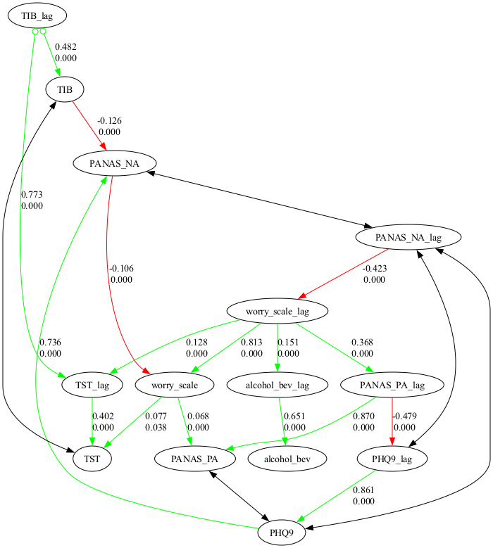
e. Show the causal graph
graph.show_graph()
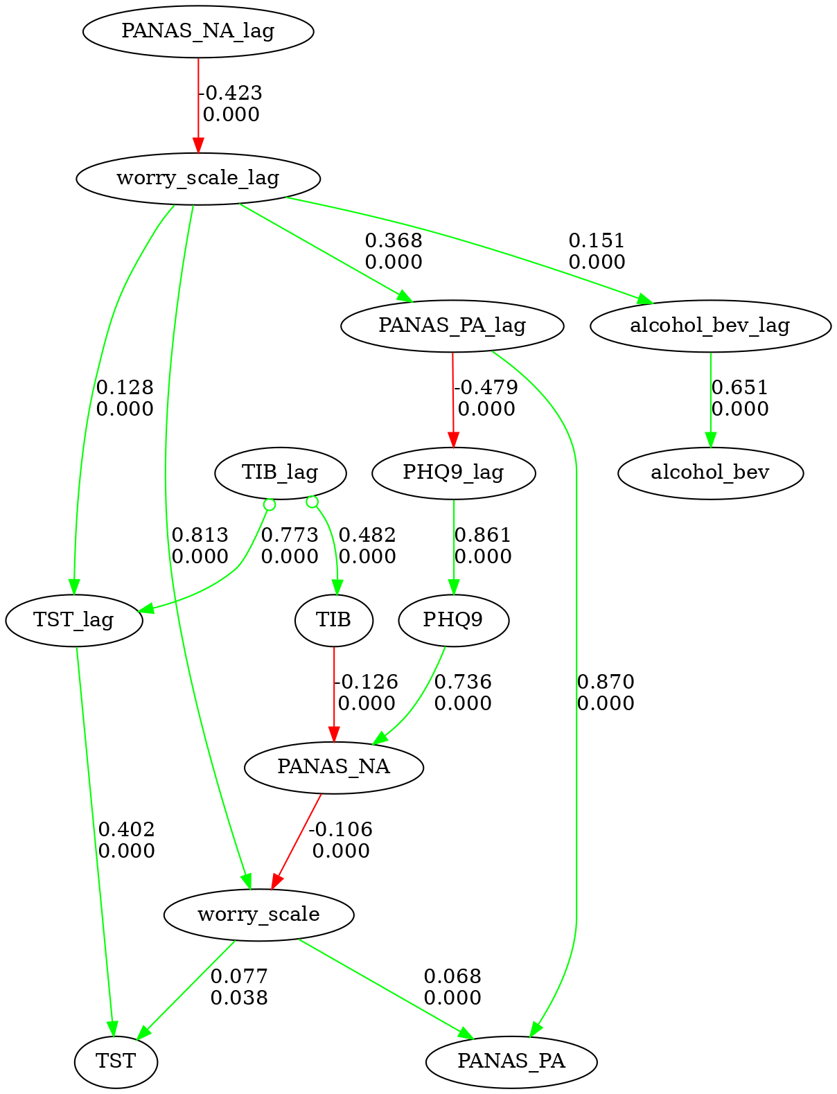
f. Show directed edges only
# lets show the directed edges only
graph.show_graph(directed_only=True)
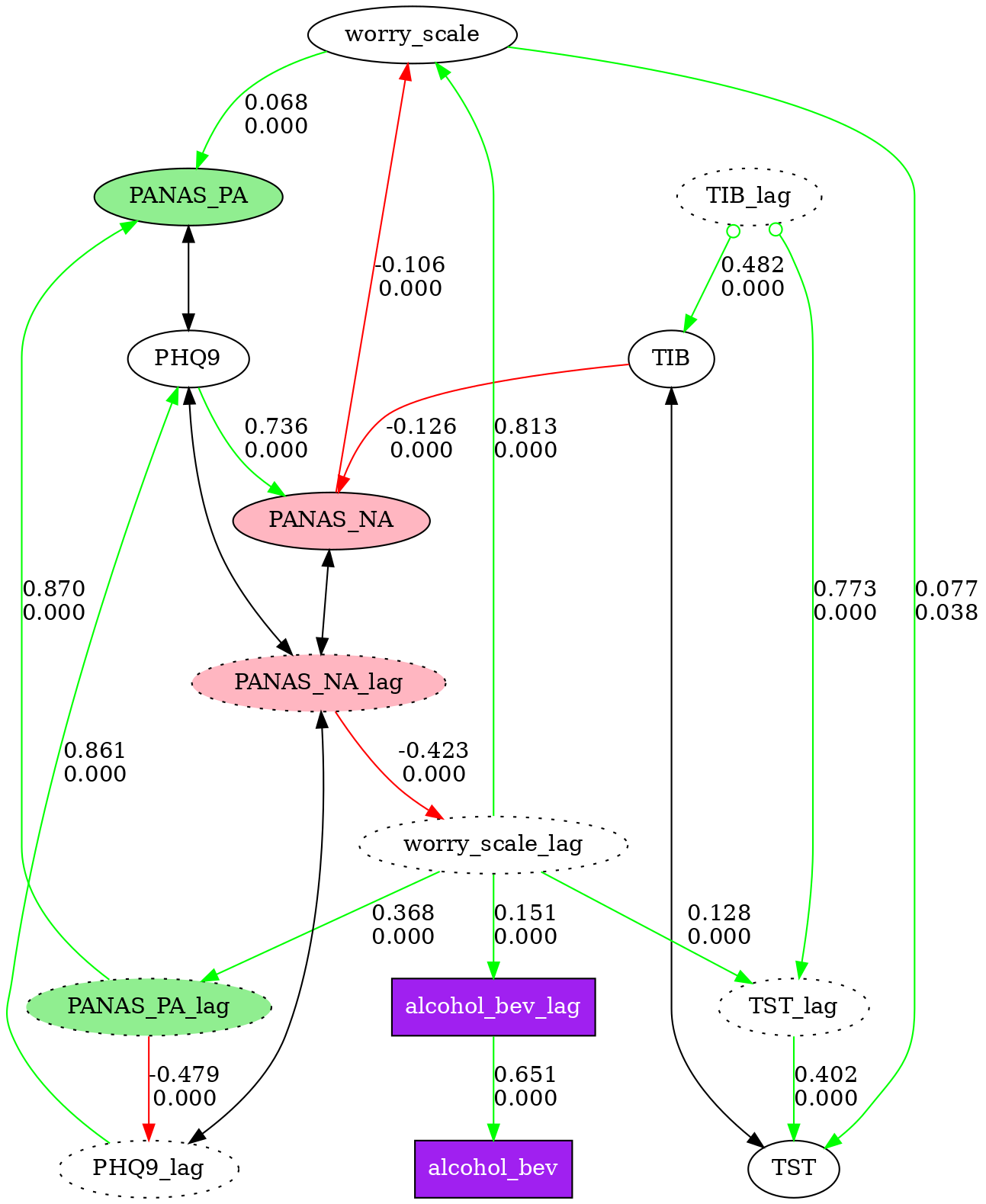
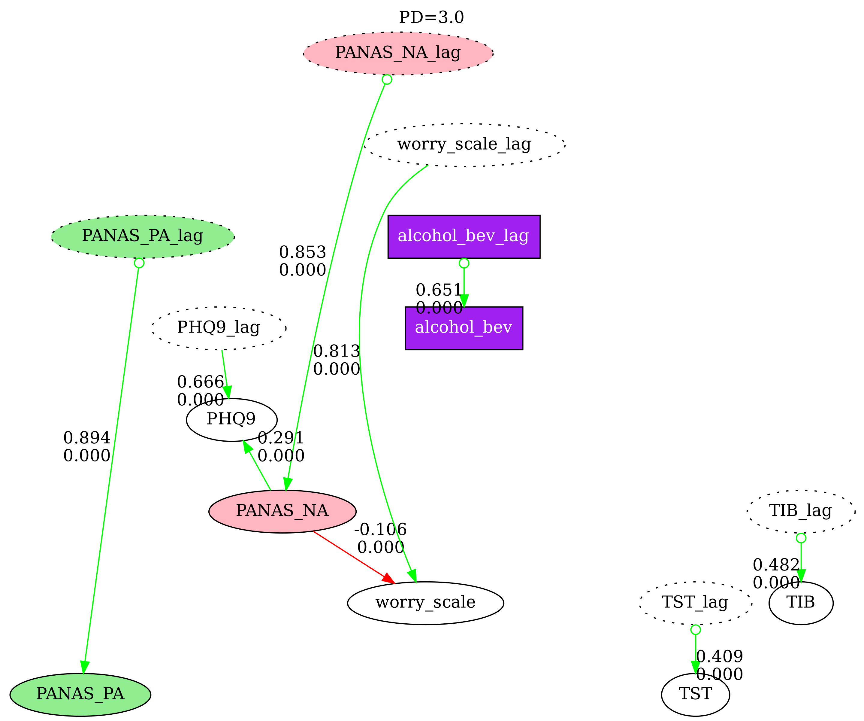
4. Node Styling
Nodes in causal graphs can be visually styled by name pattern. Define a list of style rules, each with a pattern (fnmatch glob) and any Graphviz node attributes. Rules apply in order — later rules override earlier ones for the same node.
Any valid Graphviz node attribute works: shape, fillcolor, style, color, penwidth, fontname, fontsize, etc.
node_styles = [
    {"pattern": "*_lag",        "style": "dotted"},
    {"pattern": "PANAS_PA*",    "style": "filled", "fillcolor": "lightgreen"},
    {"pattern": "PANAS_NA*",    "style": "filled", "fillcolor": "lightpink"},
    {"pattern": "PANAS_PA_lag", "style": "filled,dotted", "fillcolor": "lightgreen"},
    {"pattern": "PANAS_NA_lag", "style": "filled,dotted", "fillcolor": "lightpink"},
    {"pattern": "alcohol_bev*", "shape": "box", "style": "filled", "fillcolor": "purple", "fontcolor": "white"},
]

# Display styled graph in notebook (instead of graph.show_graph())
fc.show_styled_graph(graph, node_styles)

# Save styled graph to file (instead of graph.save_graph())
fc.save_styled_graph(graph, node_styles, "my_graph")
See fastcda_demo_short.ipynb for a complete working example.
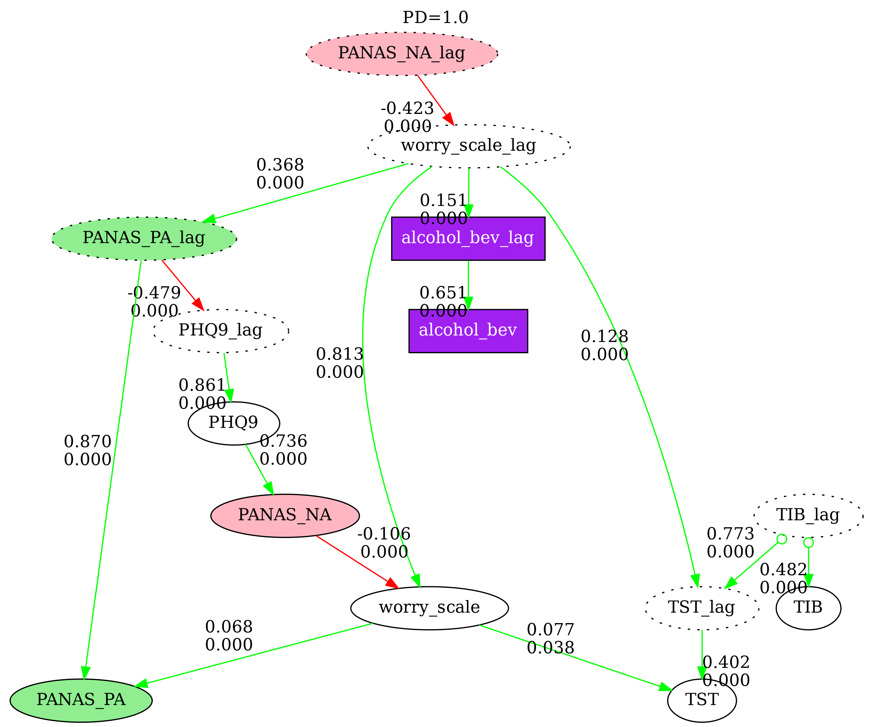
5. Multi-Graph Comparison
Compare N causal graphs side-by-side with nodes pinned at the same positions. This is useful for examining how different search parameters affect the discovered graph. Disconnected nodes (those with no edges in a particular graph) are grayed out by default.
# Run searches with different penalty discounts
result1, graph1 = fc.run_model_search(df_lag_std, model='gfci',
    score={'sem_bic': {'penalty_discount': 1.0}},
    test={"fisher_z": {"alpha": .01}}, knowledge=knowledge)

result2, graph2 = fc.run_model_search(df_lag_std, model='gfci',
    score={'sem_bic': {'penalty_discount': 2.0}},
    test={"fisher_z": {"alpha": .01}}, knowledge=knowledge)

result3, graph3 = fc.run_model_search(df_lag_std, model='gfci',
    score={'sem_bic': {'penalty_discount': 3.0}},
    test={"fisher_z": {"alpha": .01}}, knowledge=knowledge)

# Display in notebook with directed edges only
fc.show_n_graphs(
    [graph1, graph2, graph3],
    node_styles=node_styles,
    gray_disconnected=True,
    directed_only=True,
    labels=["PD=1.0", "PD=2.0", "PD=3.0"],
    graph_size="10,8"
)

# Save to files
fc.save_n_graphs(
    [graph1, graph2, graph3],
    ["graph_pd1", "graph_pd2", "graph_pd3"],
    node_styles=node_styles,
    gray_disconnected=True,
    directed_only=True,
    labels=["PD=1.0", "PD=2.0", "PD=3.0"],
    graph_size="10,8",
    res=300
)
| PD=1.0 | PD=2.0 | PD=3.0 |
|---|---|---|
 |
 |
 |
See fastcda_demo_short.ipynb for the full working example.
Release history Release notifications | RSS feed


Download files
Download the file for your platform. If you're not sure which to choose, learn more about installing packages.
Source Distribution
Built Distribution
Filter files by name, interpreter, ABI, and platform.
If you're not sure about the file name format, learn more about wheel file names.
Copy a direct link to the current filters
File details
Details for the file fastcda-0.1.24.tar.gz.
File metadata
- Download URL: fastcda-0.1.24.tar.gz
- Upload date:
- Size: 77.6 MB
- Tags: Source
- Uploaded using Trusted Publishing? No
- Uploaded via: twine/6.1.0 CPython/3.12.3
File hashes
| Algorithm | Hash digest | |
|---|---|---|
| SHA256 |
4eed18be51c62637cbe82083b92c3528a5c3463099f94cb1ae6efac26e2f192e
|
|
| MD5 |
fd21c5c3b69e0086e21f144d70387d0e
|
|
| BLAKE2b-256 |
6e30fa16976db382e4a4a575cb7d31d23f17fddab1e2f244a2235a8ad8b3569a
|
File details
Details for the file fastcda-0.1.24-py3-none-any.whl.
File metadata
- Download URL: fastcda-0.1.24-py3-none-any.whl
- Upload date:
- Size: 77.6 MB
- Tags: Python 3
- Uploaded using Trusted Publishing? No
- Uploaded via: twine/6.1.0 CPython/3.12.3
File hashes
| Algorithm | Hash digest | |
|---|---|---|
| SHA256 |
4dd93a66ff59ea281d096d0ad06496b084ff60e3c42a8cd28a3f501376687129
|
|
| MD5 |
926e8234ca88ec3c2b29105e78970831
|
|
| BLAKE2b-256 |
a5d4511e378d80d9d4fc0988fd3bd99f0bdaa3302ad1341b05c3bc55232844b5
|


