
FastWoe: Fast Weight of Evidence (WOE) Encoding and Inference






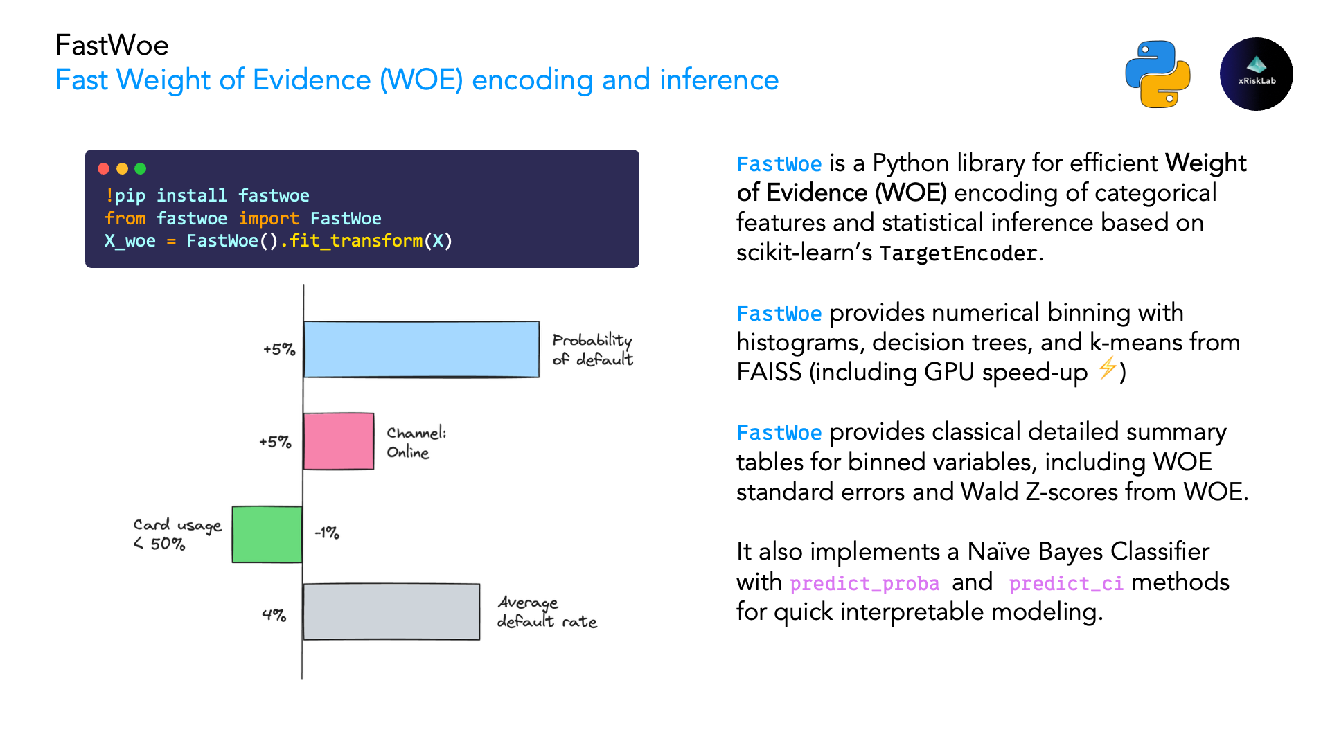
FastWoe is a Python library for efficient Weight of Evidence (WOE) encoding of categorical features and statistical inference. It's designed for machine learning practitioners seeking robust, interpretable feature engineering and likelihood-ratio-based inference for binary and multiclass classification problems.
🌟 Key Features
- Fast WOE Encoding: Leverages scikit-learn's
TargetEncoderfor efficient computation - Multiclass Support: One-vs-rest WOE encoding for targets with 3+ classes
- Statistical Confidence Intervals: Provides standard errors and confidence intervals for WOE values
- IV Standard Errors: Statistical significance testing for Information Value with confidence intervals
- Cardinality Control: Built-in preprocessing to handle high-cardinality categorical features
- Intelligent Numerical Binning: Support for traditional binning, decision tree-based binning, and FAISS KMeans clustering
- Monotonic Constraints: Enforce business logic constraints for credit scoring and regulatory compliance
- Binning Summaries: Feature-level binning statistics including Gini score and Information Value (IV)
- Compatible with scikit-learn: Follows scikit-learn's preprocessing transformer interface
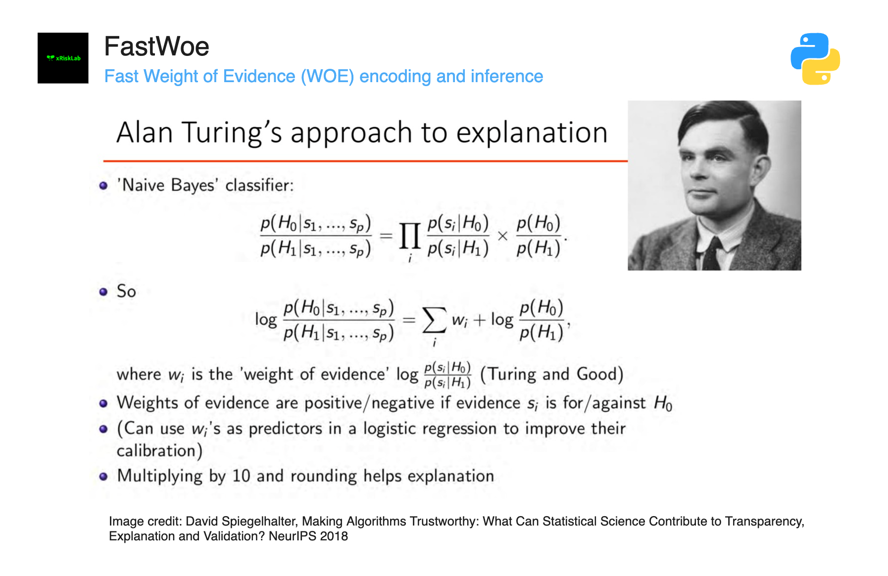
- Uncertainty Quantification: Combines Alan Turing's factor principle with Maximum Likelihood theory (see paper)
🎲 What is Weight of Evidence?
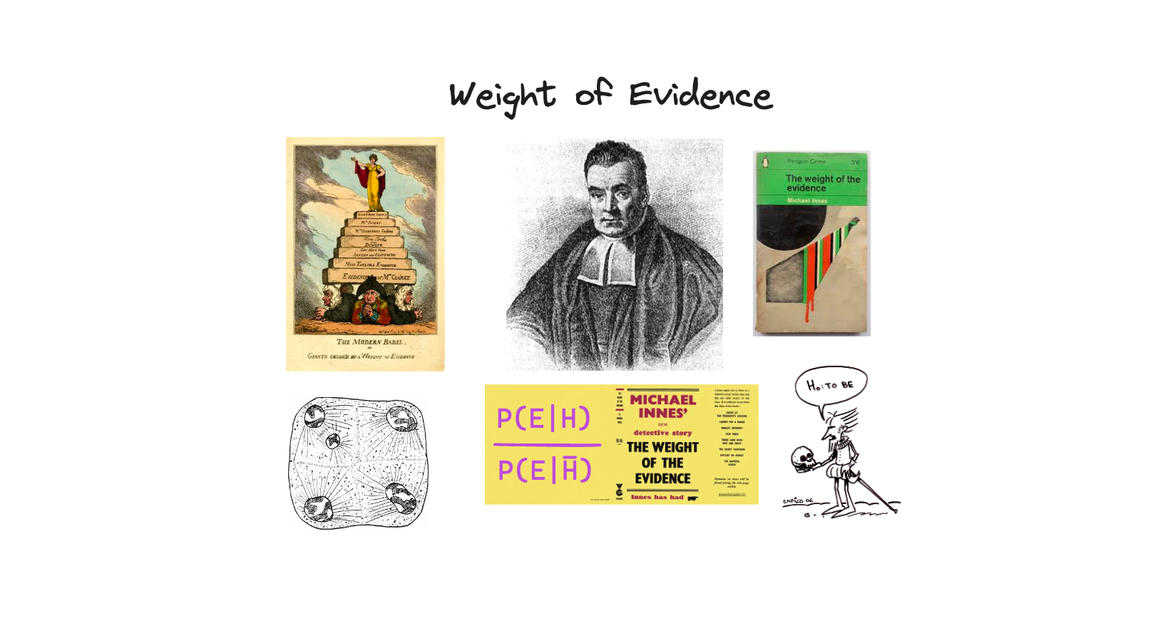
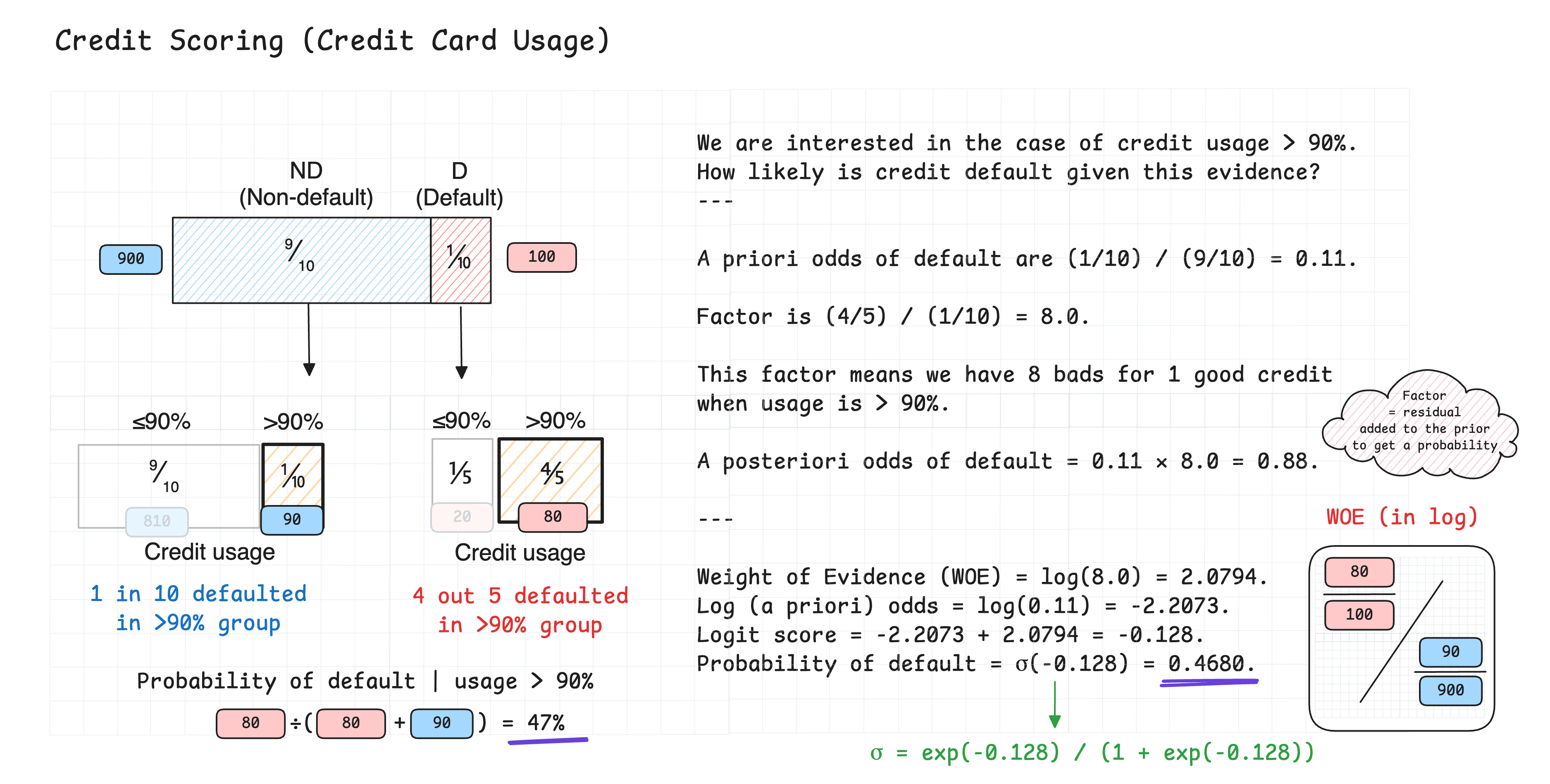
Weight of Evidence (WOE) is a statistical technique that:
- Transforms discrete features into logarithmic scores
- Measures the strength of relationship between feature categories and true labels
- Provides interpretable coefficients as weights in logistic regression models
- Handles missing values and rare categories gracefully
Mathematical Definition:
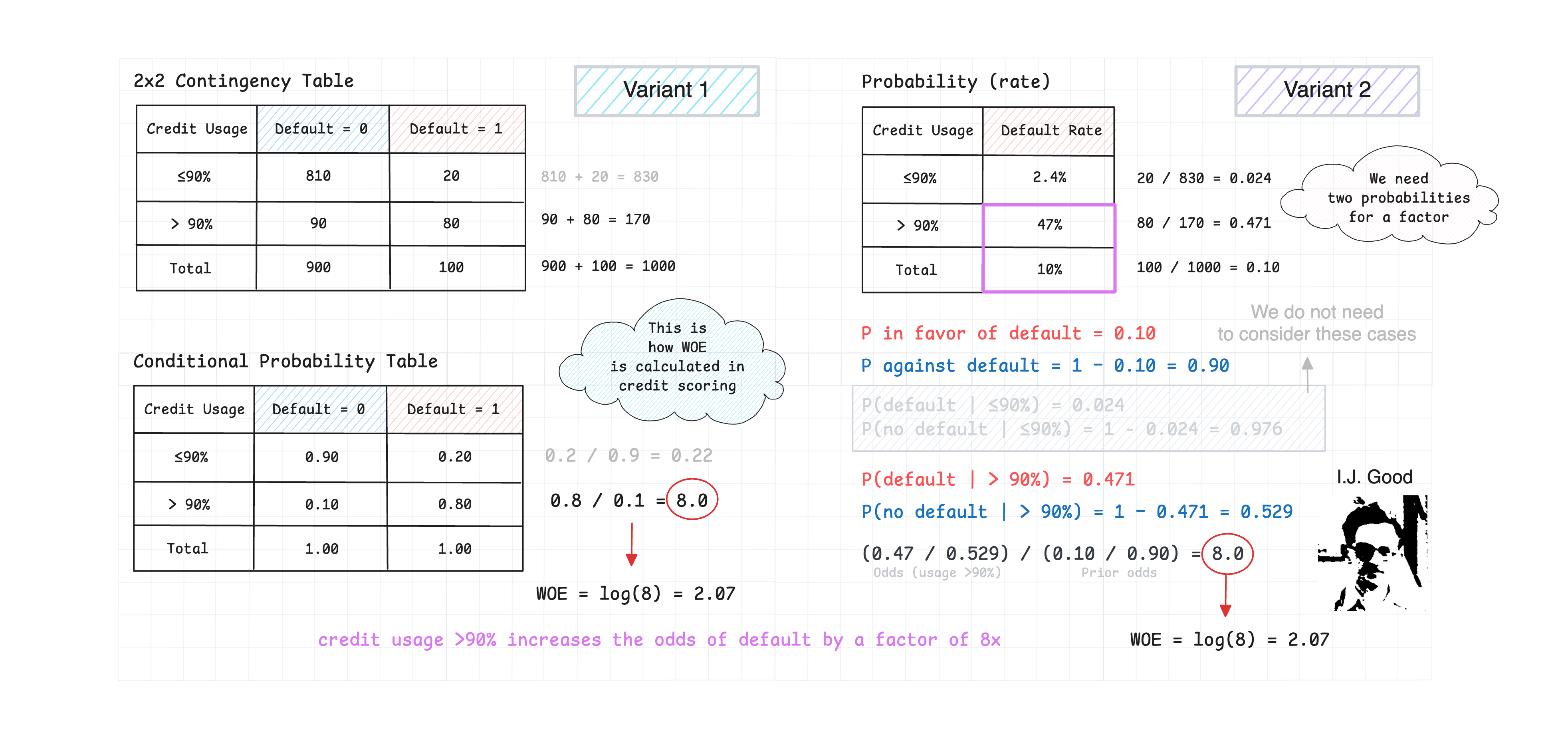
WOE = ln(P(Event|Category) / P(Non-Event|Category)) - ln(P(Event) / P(Non-Event))
Where WOE represents the log-odds difference between a category and the overall population.
🚀 Installation
From PyPI (Recommended)
pip install fastwoe
📦 View on PyPI: https://pypi.org/project/fastwoe/
Optional Dependencies
FAISS KMeans Binning
Optional: FAISS for KMeans clustering-based binning (see Numerical Feature Binning):
# CPU version (recommended for most users)
pip install fastwoe[faiss]

# GPU version (for CUDA-enabled systems)
pip install fastwoe[faiss-gpu]
For GPU acceleration support:
pip install faiss-gpu # Requires CUDA
⚠️ Important: If you get
ImportError: FAISS is required for faiss_kmeans binning method, you need to install the[faiss]extras. See FAISS Troubleshooting Guide for detailed solutions.
WebAssembly (Pyodide)
FastWoe runs in Pyodide (e.g. JupyterLite): await micropip.install("fastwoe"). numba has no WebAssembly build, so it is not installed there and the Somers' D code runs as plain Python: the same calculation and results, without compilation (200,000 rows in about 1 to 3 seconds in the browser).
Plotting Support
Optional: Matplotlib for CAP curves and WOE visualization:
# For plot_performance() and visualize_woe()
pip install fastwoe[plotting]
Metrics and Plots Only
fastwoe.metrics and fastwoe.plots load without scikit-learn, so importing them is fast and does not initialise the WOE encoder:
from fastwoe.metrics import somersd_yx, gini_contributions
from fastwoe.plots import plot_performance
From Source
git clone https://github.com/xRiskLab/fastwoe.git
cd fastwoe
pip install -e .
Development Installation
git clone https://github.com/xRiskLab/fastwoe.git
cd fastwoe
pip install -e ".[dev]"
📖 Quick Start
import pandas as pd
import numpy as np
from fastwoe import FastWoe, WoePreprocessor

# Create sample data
data = pd.DataFrame({
    'category': ['A', 'B', 'C'] * 100 + ['D'] * 50,
    'high_card_cat': [f'cat_{i}' for i in np.random.randint(0, 50, 350)],
    'target': np.random.binomial(1, 0.3, 350)
})

# Step 1: Preprocess high-cardinality features (optional)
preprocessor = WoePreprocessor(max_categories=10, min_count=5)
X_preprocessed = preprocessor.fit_transform(
    data[['category', 'high_card_cat']],
    cat_features=['high_card_cat']  # Only preprocess this column
)

# Step 2: Apply WOE encoding
woe_encoder = FastWoe()
X_woe = woe_encoder.fit_transform(X_preprocessed, data['target'])

print("WOE-encoded features:")
print(X_woe.head())

# Step 3: Get detailed mappings with statistics
mapping = woe_encoder.get_mapping('category')
print("\nWOE Mapping for 'category':")
print(mapping[['category', 'count', 'event_rate', 'woe', 'woe_se']])
🎯 Multiclass Support
FastWoe now supports multiclass classification using a one-vs-rest approach! For targets with 3+ classes, FastWoe automatically creates separate WOE encodings for each class against all others.
Multiclass Example
import pandas as pd
import numpy as np
from fastwoe import FastWoe
from sklearn.ensemble import RandomForestClassifier
from sklearn.metrics import classification_report

# Create multiclass data
X = pd.DataFrame({
    'job': ['teacher', 'engineer', 'artist', 'doctor'] * 25,
    'age_group': ['<30', '30-50', '50+'] * 33 + ['<30'],
    'income': np.random.normal(50000, 20000, 100),
})
y = pd.Series([0, 1, 2, 0, 1] * 20)  # 3 classes

# Fit FastWoe with multiclass target
woe_encoder = FastWoe()
woe_encoder.fit(X, y)

# Transform data - creates multiple columns per feature
X_woe = woe_encoder.transform(X)
print(f"Original features: {X.shape[1]}")
print(f"WOE features: {X_woe.shape[1]}")  # 3x more columns
print(f"Column names: {list(X_woe.columns)}")
# Output: ['job_class_0', 'job_class_1', 'job_class_2', 'age_group_class_0', ...]

# Get probabilities for all classes
probs = woe_encoder.predict_proba(X)
print(f"Probabilities shape: {probs.shape}")  # (n_samples, n_classes)

# Get class-specific probabilities
class_0_probs = woe_encoder.predict_proba_class(X, class_label=0)
class_1_probs = woe_encoder.predict_proba_class(X, class_label=1)

# Get confidence intervals for specific class
class_0_ci = woe_encoder.predict_ci_class(X, class_label=0)
print(f"Class 0 CI shape: {class_0_ci.shape}")  # (n_samples, 2) [lower, upper]

# Train a classifier on WOE features
rf = RandomForestClassifier(n_estimators=100, random_state=42)
rf.fit(X_woe, y)
predictions = rf.predict(X_woe)

print("\nClassification Report:")
print(classification_report(y, predictions))
Multiclass Features
- One-vs-Rest Encoding: Each class gets separate WOE scores against all others
- Class-Specific Methods:
predict_proba_class()andpredict_ci_class()for individual classes - Softmax Probabilities:
predict_proba()returns probabilities that sum to 1 across classes - Comprehensive Statistics: All existing methods work with multiclass (IV analysis, feature stats, etc.)
- String Labels: Supports both integer and string class labels
Class-Specific Predictions
# Method 1: Extract from full results
all_probs = woe_encoder.predict_proba(X)
class_0_probs = all_probs[:, 0]  # Extract class 0

# Method 2: Use class-specific methods (recommended)
class_0_probs = woe_encoder.predict_proba_class(X, class_label=0)
class_0_ci = woe_encoder.predict_ci_class(X, class_label=0)

# Practical usage examples
high_risk_mask = woe_encoder.predict_proba_class(X, class_label=0) > 0.5
high_confidence_mask = woe_encoder.predict_ci_class(X, class_label=2)[:, 0] > 0.3
🔧 Advanced Usage
Probability Predictions
# Get predictions with Naive Bayes classification
preds = woe_encoder.predict_proba(X_preprocessed)[:, 1]
print(preds.mean())
Confidence Intervals
# Get predictions with confidence intervals
ci_results = woe_encoder.predict_ci(X_preprocessed, alpha=0.05)
print(ci_results[['prediction', 'lower_ci', 'upper_ci']].head())
Feature Statistics
# Get comprehensive feature statistics
feature_stats = woe_encoder.get_feature_stats()
print(feature_stats)
Information Value (IV) Standard Errors
FastWoe provides statistical rigor for Information Value calculations with confidence intervals and significance testing.
We can calculate the standard error of IV for each feature using the get_iv_analysis method.
# Get IV analysis with confidence intervals
iv_analysis = woe_encoder.get_iv_analysis()
print(iv_analysis)
Output:
       feature     iv  iv_se  iv_ci_lower  iv_ci_upper  iv_pvalue iv_significance
strong_feature 0.1571 0.0283       0.1016       0.2126     0.0000     Significant
  weak_feature 0.0035 0.0042       0.0000       0.0117     0.4454 Not Significant
iv_seis the delta-method standard error with both the WOE values and the weights(b - g)treated as estimated:Var(IV) = Var_B(WOE - g/b)/n_bad + Var_G(WOE + b/g)/n_good. Holding the weights fixed understates it by about half.iv_pvaluetests IV = 0 with a chi-square test: under no predictive power,n_eff * IV ~ chi2(k - 1)withn_eff = n_bad * n_good / (n_bad + n_good)(computed as Pearson's X², which stays finite for bins holding one class).iv_significanceisp < alpha. A normal testIV / SEdoes not work here: IV is never negative and is not normal near 0.- Noise has positive IV. Under no predictive power,
E[IV] ≈ (k - 1) / n_eff:weak_featureabove (IV 0.0035, p = 0.45) is at that level. Many bins and few bads raise it.
Additionally, we can calculate the standard error of IV for a specific feature using the get_iv_analysis method.
# Get IV analysis for a specific feature
single_feature_iv = woe_encoder.get_iv_analysis('feature_name')

# All feature statistics now include IV standard errors
feature_stats = woe_encoder.get_feature_stats()
# Contains: iv, iv_se, iv_ci_lower, iv_ci_upper columns
Transform Output Modes
X_woe = woe_encoder.transform(X_preprocessed)                          # WOE values (default)
X_norm = woe_encoder.transform(X_preprocessed, output='woe_norm')       # Normalized WOE (WOE / SE)
X_wald = woe_encoder.transform(X_preprocessed, output='wald')           # Wald statistic
X_upper = woe_encoder.transform(X_preprocessed, output='woe_upper_ci')  # Upper 95% CI
X_lower = woe_encoder.transform(X_preprocessed, output='woe_lower_ci')  # Lower 95% CI
Unseen Categories and Missing Values
A category absent at fit time, including a missing value in a numeric feature that had no missing values in training, has no learned weight and is encoded as WOE 0 (the prior odds). FastWoe(unseen=...) controls what happens then:
FastWoe(unseen="warn")   # default: encode as WOE 0 and warn with column and counts
FastWoe(unseen="prior")  # encode as WOE 0 silently
FastWoe(unseen="raise")  # fail, e.g. for validation runs
woe_encoder.unseen_counts_  # {column: {category: count}} from the last transform
Fit on data that contains missing values so a Missing bin is learned.
Conditional WOE
Summing marginal WOE is exact only when features are independent. Conditional WOE uses Good's chain rule, W(H : E1 E2) = W(H : E1) + W(H : E2 | E1), so each weight is measured within the population picked out by the features before it (binary targets only):
woe = FastWoe(conditional=True)             # conditions in X's column order
woe.fit(X[["delinquent", "high_util"]], y)

woe.transform(X)          # per-feature conditional weights; they sum to the score
woe.predict_proba(X)      # no double counting of shared signal
woe.predict_ci(X)         # SE of the joint cell, not a sum of per-feature variances
woe.get_mapping("high_util")  # weight of each category *given* each earlier value
woe.get_iv_analysis()         # marginal iv plus iv_conditional: what each feature adds given the earlier ones
print(woe.export_text())      # the weights as a tree, like sklearn's export_text
Conditional WOE tree  ·  target: default  ·  event rate = share of rows with default = 1
Conditioning order: delinquent → high_util  ·  prior log-odds -1.997

                            W  95% interval           n  event rate  -0.46  0                 +1.35
root                                             20,000       11.9%
├── delinquent = 0     -0.403  [-0.458, -0.349]  17,021        8.3%  ─●─    ┊
│   ├── high_util = 0  -0.073  [-0.136, -0.010]  13,636        7.8%       ─●─
│   └── high_util = 1  +0.256  [+0.146, +0.366]   3,385       10.5%         ┊  ─●──
└── delinquent = 1     +1.277  [+1.200, +1.353]   2,979       32.7%         ┊                   ─●─
    ├── high_util = 0  -0.255  [-0.381, -0.129]   1,220       27.4%   ──●── ┊
    └── high_util = 1  +0.164  [+0.067, +0.261]   1,759       36.4%         ┊──●──
Each node shows its conditional weight W with a 95% interval, its size and its event rate (share of rows with target = 1). The bars draw the intervals on one shared scale with a zero line (┼ where an interval covers zero), so weights can be compared at a glance; ○ [fallback] marks cells that used the marginal weight. max_depth= truncates deep trees and bar_width=0 hides the bars.
On two correlated features, an applicant who is delinquent with high utilisation:
| delinquent | high_util | P(bad) | |
|---|---|---|---|
| Marginal WOE | 1.277 | 0.571 | 0.463 |
| Conditional, delinquent first | 1.277 | 0.164 | 0.364 |
| Conditional, high_util first | 0.870 | 0.571 | 0.364 |
| Observed rate in that cell | 0.364 |
The order (conditional_order=[...]) changes how weight is attributed across features, not the score. Conditioning cells multiply with each feature, so this suits a short list of correlated features rather than a whole scorecard: cells with fewer than conditional_min_count (default 30) bads or goods fall back to the marginal weight and are listed in conditional_fallbacks_. With two features the score stays order-invariant even then; with three or more, fallbacks are where the order can change the score.
Information Value follows the same chain rule. get_iv_analysis() keeps iv as the marginal IV and adds iv_conditional (with SE, confidence interval, significance and conditioned_on): the IV a feature adds given the features before it. Conditional IVs sum to the joint IV of the features, so a correlated feature that looks strong on its own can show a small, non-significant conditional IV.
The order is an attribution choice: when the per-feature weights or IVs are used for explanations, set conditional_order deliberately (e.g. cause before symptom) and document it.
A worked example, including calibration against marginal WOE and logistic regression, fallbacks and explanations, is in examples/notebooks/fastwoe_conditional.ipynb.
Numerical Feature Binning
FastWoe supports three methods for binning numerical features:
1. Histogram-Based Binning
# Use KBinsDiscretizer with quantile strategy
woe_encoder = FastWoe(
    binning_method="kbins",
    binner_kwargs={
        "n_bins": 5,
        "strategy": "quantile",  # or "uniform", "kmeans"
        "encode": "ordinal"
    }
)
2. Decision Tree-Based Binning
# Use single decision tree to find optimal splits
woe_encoder = FastWoe(
    binning_method="tree",
    tree_kwargs={
        "max_depth": 3,
        "min_samples_split": 20,
        "min_samples_leaf": 10
    }
)

# Or use a custom tree estimator
from sklearn.tree import ExtraTreeClassifier
woe_encoder = FastWoe(
    binning_method="tree",
    tree_estimator=ExtraTreeClassifier,
    tree_kwargs={"max_depth": 2, "random_state": 42}
)
3. FAISS KMeans Binning
# Use FAISS KMeans clustering for efficient binning
# First install FAISS: pip install fastwoe[faiss] (CPU) or fastwoe[faiss-gpu] (GPU)
woe_encoder = FastWoe(
    binning_method="faiss_kmeans",
    faiss_kwargs={
        "k": 5,              # Number of clusters
        "niter": 20,         # Number of iterations
        "verbose": False,    # Show progress
        "gpu": False         # Use GPU acceleration (requires faiss-gpu)
    }
)

# Example with GPU acceleration
woe_encoder = FastWoe(
    binning_method="faiss_kmeans",
    faiss_kwargs={
        "k": 8,
        "niter": 50,
        "verbose": True,
        "gpu": True          # pip install faiss-gpu-cu12 for CUDA 12
    }
)
Benefits of FAISS KMeans Binning:
- Efficient Clustering: Uses Facebook's FAISS library for fast KMeans clustering
- Data-Driven Bins: Creates bins based on feature value clusters, not quantiles
- GPU Acceleration: Optional GPU support for large datasets
- Scalable: Optimized for high-dimensional and large-scale data
- Meaningful Labels: Generates interpretable bin labels based on cluster centroids
- Missing Value Handling: Properly handles missing values in clustering
Benefits of Tree-Based Binning:
- Target-Aware: Splits are optimized for the target variable
- Non-Linear Relationships: Captures complex patterns better than uniform/quantile binning
- Automatic Bin Count: Number of bins determined by tree structure
- Flexible Configuration: Use any tree estimator with custom hyperparameters
Pipeline Integration
from sklearn.pipeline import Pipeline
from sklearn.linear_model import LogisticRegression

# Create a complete pipeline
pipeline = Pipeline([
    ('preprocessor', WoePreprocessor(top_p=0.95, min_count=10)),
    ('woe_encoder', FastWoe()),
    ('classifier', LogisticRegression())
])

# Fit the entire pipeline
pipeline.fit(data[['category', 'high_card_cat']], data['target'])
🎯 Monotonic Constraints for Credit Scoring
FastWoe supports monotonic constraints for numerical features, ensuring that WOE values follow business logic requirements. This is particularly important for credit scoring and regulatory compliance.
When to Use Monotonic Constraints
- Credit Scoring: Higher income should lead to lower risk
- Age-based Risk: Higher age might lead to higher risk (depending on context)
- Credit Score: Higher credit scores should lead to lower risk
- Regulatory Compliance: When business rules require monotonic relationships
Example Usage
import pandas as pd
import numpy as np
from fastwoe import FastWoe

# Create sample credit scoring data
np.random.seed(42)
n_samples = 1000

# Income: higher income -> lower risk (decreasing constraint)
income = np.random.lognormal(mean=10, sigma=0.5, size=n_samples)
income_risk = 1 / (1 + np.exp((income - np.median(income)) / 20))

# Age: higher age -> higher risk (increasing constraint)
age = np.random.normal(35, 12, n_samples)
age_risk = 1 / (1 + np.exp(-(age - 35) / 8))

# Credit score: higher score -> lower risk (decreasing constraint)
credit_score = np.random.normal(650, 100, n_samples)
credit_score = np.clip(credit_score, 300, 850)
credit_risk = 1 / (1 + np.exp((credit_score - 650) / 50))

# Combine risks
combined_risk = (income_risk + age_risk + credit_risk) / 3
y = (combined_risk > 0.5).astype(int)

X = pd.DataFrame({
    'income': income,
    'age': age,
    'credit_score': credit_score
})

# Apply monotonic constraints
woe_encoder = FastWoe(
    binning_method="tree",
    monotonic_cst={
        "income": -1,        # Decreasing: higher income -> lower risk
        "age": 1,            # Increasing: higher age -> higher risk
        "credit_score": -1   # Decreasing: higher score -> lower risk
    },
    numerical_threshold=10
)

woe_encoder.fit(X, y)

# Check that constraints were applied
summary = woe_encoder.get_binning_summary()
print(summary[['feature', 'monotonic_constraint']])
Constraint Values
1: Increasing constraint (higher values → higher risk)-1: Decreasing constraint (higher values → lower risk)0: No constraint (default)
Important Notes
- Tree method: Uses native scikit-learn monotonic constraints
- KBins & FAISS methods: Uses isotonic regression to enforce constraints
- Multiclass Support: Monotonic constraints work with multiclass targets - constraints are applied independently to each class's WOE values
- Constraints ensure WOE values follow the specified monotonic pattern
- Performance may be slightly different but more interpretable
- Essential for regulatory compliance in credit scoring
For a complete example, see examples/scripts/fastwoe_monotonic.py.
📋 API Reference
FastWoe Class
Parameters
encoder_kwargs(dict): Additional parameters for sklearn's TargetEncoderrandom_state(int): Random state for reproducibilitybinning_method(str): Method for numerical binning - "kbins" (default), "tree", or "faiss_kmeans"binner_kwargs(dict): Parameters for KBinsDiscretizer (when binning_method="kbins")tree_estimator(estimator): Custom tree estimator for binning (when binning_method="tree")tree_kwargs(dict): Parameters for tree estimatorfaiss_kwargs(dict): Parameters for FAISS KMeans (when binning_method="faiss_kmeans")monotonic_cst(dict): Monotonic constraints for numerical features. Maps feature names to constraint values: 1 (increasing), -1 (decreasing), 0 (no constraint). Supported with all binning methods: tree (native), kbins/faiss_kmeans (isotonic regression). Works with binary and multiclass targets.
Key Methods
fit(X, y): Fit the WOE encodertransform(X): Transform features to WOE valuesfit_transform(X, y): Fit and transform in one stepget_mapping(column): Get WOE mapping for specific columnpredict_proba(X): Get probability predictionspredict_ci(X, alpha): Get predictions with confidence intervals
WoePreprocessor Class
The WoePreprocessor is a preprocessing step that reduces the cardinality of categorical features. It is used to handle high-cardinality categorical features.
Parameters
max_categories(int): Maximum categories to keep per featuretop_p(float): Keep categories covering top_p% of frequencymin_count(int): Minimum count required for categoryother_token(str): Token for grouping rare categories
Key Methods
fit(X, cat_features): Fit preprocessortransform(X): Apply preprocessingget_reduction_summary(X): Get cardinality reduction statistics
Example: Using top_p parameter
# Dataset with 100 categories:
# "A" (40%), "B" (30%), "C" (15%), "D" (10%), remaining 96 categories (5% total)

preprocessor = WoePreprocessor(top_p=0.95, min_count=5)
# Result: Keeps ["A", "B", "C", "D"] (95% coverage), groups rest as "__other__"
# Reduces 100 → 5 categories while preserving 95% of the categories
WeightOfEvidence Class
The WeightOfEvidence class provides interpretability for FastWoe classifiers with automatic parameter inference and uncertainty quantification through confidence intervals.
Parameters
classifier(FastWoe, optional): FastWoe classifier to explain (auto-created if None)X_train(array-like, optional): Training features (auto-inferred if possible)y_train(array-like, optional): Training labels (auto-inferred if possible)feature_names(list, optional): Feature names (auto-inferred if possible)class_names(list, optional): Class names (auto-inferred if possible)auto_infer(bool): Enable automatic parameter inference (default=True)
Key Methods
explain(x, sample_idx=None, class_to_explain=None, true_label=None, return_dict=True): Explain single sample or sample from datasetexplain_ci(x, sample_idx=None, alpha=0.05, return_dict=True): Explain with confidence intervals for uncertainty quantificationpredict_ci(X, alpha=0.05): Batch predictions with confidence boundssummary(): Get explainer overview and statistics
Key Features
- Auto-Inference: Automatically detects parameters from FastWoe classifiers
- Dual Usage: Support both
explain(sample)andexplain(dataset, index)patterns - Uncertainty Quantification: Confidence intervals for WOE scores and probabilities
- Rich Output: Human-readable interpretations with evidence strength levels
📊 Theoretical Background
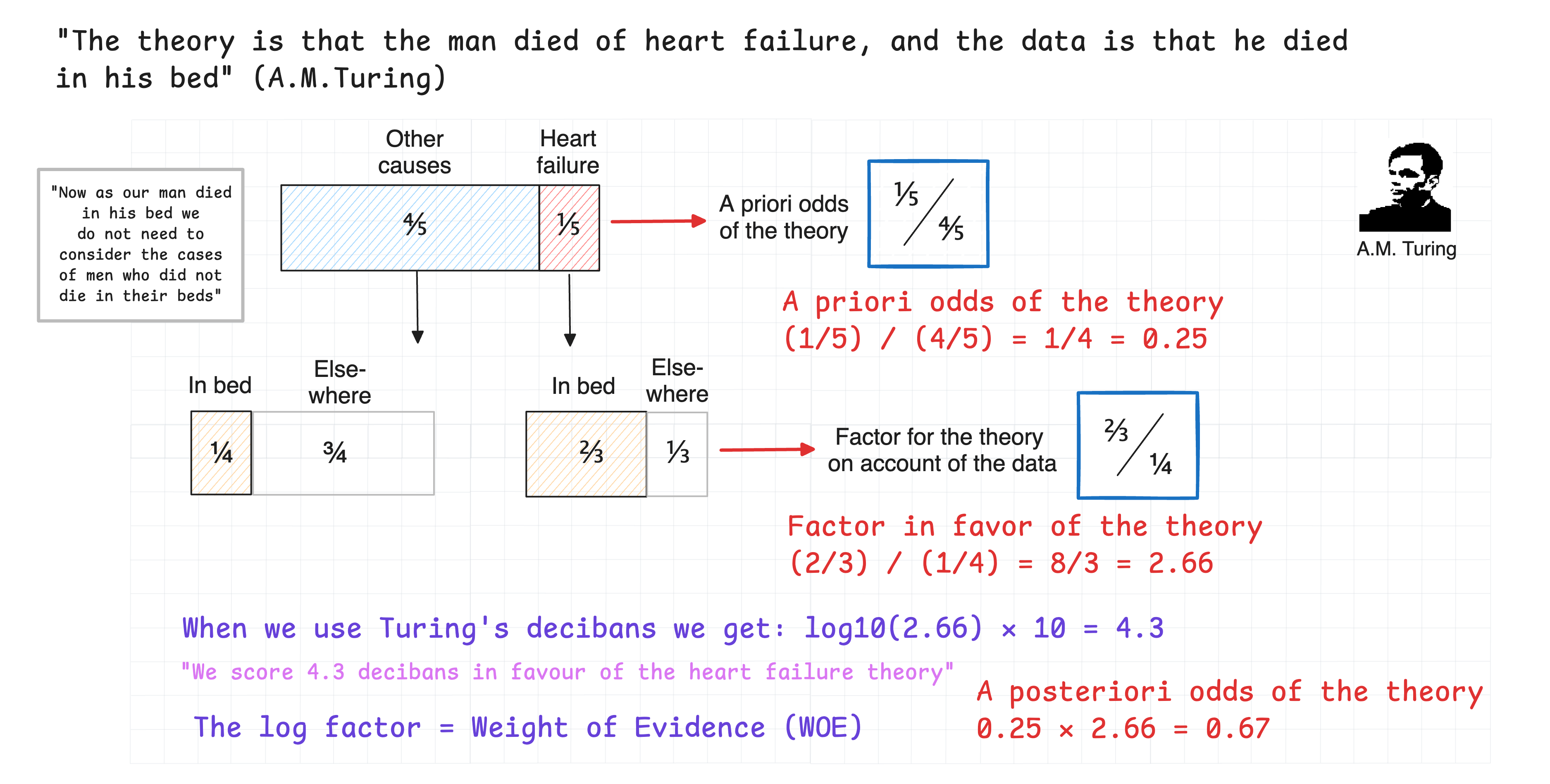
This implementation is based on rigorous statistical theory:
- WOE Standard Error:
SE(WOE) = sqrt(1/good_count + 1/bad_count) - Confidence Intervals: Using normal approximation with calculated standard errors
- Information Value: Measures predictive power of each feature
- Gini Score: Derived from AUC to measure discriminatory power
For rare counts, we rely on the rule of three to calculate the standard error.
For technical details, see Weight of Evidence (WOE), Log Odds, and Standard Errors.
🧪 Testing
Run the test suite:
# Install test dependencies
pip install -e ".[dev]"

# Run tests
pytest

# Run tests with coverage
pytest --cov=fastwoe --cov-report=html
🛠️ Development
Development Setup
Clone the repository and install dependencies:
git clone https://github.com/xRiskLab/fastwoe.git
cd fastwoe
uv sync --dev
Running Tests
Run the main test suite:
uv run pytest
Run tests without slow compatibility tests:
uv run pytest -m "not slow"
Run compatibility tests across Python/scikit-learn versions (requires uv):
uv run pytest -m compatibility
Run specific test categories:
# Only fast compatibility checks
uv run pytest -m "compatibility and not slow"

# Only slow cross-version tests
uv run pytest -m "compatibility and slow"
Code Quality and Type Checking
FastWoe uses several tools to maintain code quality:
# Format code
make format

# Run linting
make lint

# Run type checking (lenient mode for pandas/numpy)
make typecheck

# Run type checking (strict mode)
make typecheck-strict

# Run all checks (format, lint, typecheck)
make check-all

# CI-friendly checks (passes with expected pandas/numpy type issues)
make ci-check
Local GitHub Actions Testing
Test your CI/CD workflows locally using act:
# Test workflows locally (dry run)
act --container-architecture linux/amd64 -W .github/workflows/ci.yml --dryrun

# Test specific jobs
act --container-architecture linux/amd64 -j lint -W .github/workflows/ci.yml --dryrun
act --container-architecture linux/amd64 -j type-check -W .github/workflows/typecheck.yml --dryrun
See Local Testing with Act for comprehensive documentation.
Type Checking Notes:
- FastWoe uses ty for type checking via
make typecheck - Many type errors are expected due to pandas/numpy dynamic typing
- CI mode treats expected pandas/numpy type issues as success
- Use
make typecheck-strictto fail on any type errors
Building the Package
Build wheel and source distribution:
uv build
Install from local build:
uv pip install dist/fastwoe-*.whl
Test installation in clean environment:
# Create temporary environment
uv venv .test-env --python 3.9
uv pip install --python .test-env/bin/python dist/fastwoe-*.whl
.test-env/bin/python -c "import fastwoe; print(f'FastWoe {fastwoe.__version__} installed successfully!')"
Code Quality
Format code:
uv run black fastwoe/ tests/
Lint code:
uv run ruff check fastwoe/ tests/
📈 Performance Characteristics
- Memory Efficient: Uses pandas and numpy for vectorized operations
- Scalable: Handles datasets with millions of rows
- Fast: Leverages sklearn's optimized TargetEncoder implementation
- Robust: Handles edge cases like single categories and missing values
📝 Changelog
For a changelog, see CHANGELOG.
🔧 Troubleshooting
FAISS Import Issues
If you encounter FAISS-related import errors, here are common solutions:
Error: No module named 'numpy._core'
- This occurs when FAISS was compiled against an older NumPy version
- Solution: Upgrade to compatible FAISS version which supports Python 3.7-3.12 and both NumPy 1.x and 2.x
- Run:
pip install --upgrade faiss-cpu>=1.12.0orpip install --upgrade faiss-gpu-cu12>=1.12.0
Error: AttributeError: module 'faiss' has no attribute 'KMeans'
- This occurs when using an older FAISS version with incorrect import paths
- Solution: The latest
fastwoe[faiss]installation handles this automatically - If using FAISS directly, import as:
from faiss.extra_wrappers import Kmeans
Error: A module that was compiled using NumPy 1.x cannot be run in NumPy 2.x
- This occurs when FAISS was compiled against NumPy 1.x but you're using NumPy 2.x
- Solution: Use compatible FAISS version which supports both NumPy versions:
- CPU:
pip install --upgrade faiss-cpu>=1.12.0 - GPU:
pip install --upgrade faiss-gpu-cu12>=1.12.0
- CPU:
- Or downgrade NumPy:
pip install "numpy<2.0"
Verification
To verify FAISS is working correctly:
from fastwoe import FastWoe
import pandas as pd
import numpy as np

# Test FAISS functionality
X = pd.DataFrame({'feature': np.random.randn(100)})
y = np.random.randint(0, 2, 100)

woe = FastWoe(binning_method='faiss_kmeans', faiss_kwargs={'k': 3})
woe.fit(X, y)  # Should work without errors
📄 License
This project is licensed under the MIT License - see the LICENSE file for details.
📚 References
- Alan M. Turing (1942). The Applications of Probability to Cryptography.
- I. J. Good (1950). Probability and the Weighing of Evidence.
- Daniele Micci-Barreca (2001). A preprocessing scheme for high-cardinality categorical attributes in classification and prediction problems.
- Naeem Siddiqi (2006). Credit Risk Scorecards: Developing and Implementing Intelligent Credit Scoring.
🔗 Other Projects
- scikit-learn: Python Machine learning library providing TargetEncoder implementation
- category_encoders: Additional categorical encoding methods
- WoeBoost: Weight of Evidence (WOE) Gradient Boosting in Python
ℹ️ Additional Information
- Documentation: README and Theoretical Background
- Examples: See examples/ directory
1 maintainer

Release files for fastwoe 0.1.9
For a detailed explanation of source distributions (sdists) and built distributions (wheels), please see the package formats documentation.
Source distribution (sdist)
| File | Size | Uploaded | |
|---|---|---|---|
| fastwoe-0.1.9.tar.gz | 145.1 kB | Details |
Built distribution (wheel)
| File | Interpreter | ABI | Platform | Reset |
|---|---|---|---|---|
| fastwoe-0.1.9-py3-none-any.whl | Python 3 | none | any | Details |
Total release size: 235.5 kB
Release files / fastwoe-0.1.9.tar.gz
| Download URL | fastwoe-0.1.9.tar.gz |
|---|---|
| Size | 145.1 kB |
| Tags | Source |
|
SHA-256 checksum How to use checksums |
e9d34c0c9649b374f49e64712f411226e09358b2c46d03c00063096361260fd0
|
|
BLAKE2b-256 checksum How to use checksums |
dde2f5134247bde8a10871876d6b1fc1e49af2c5efd89415bcc37b484dca0b74
|
| Upload date | |
|
Uploaded using Trusted Publishing? What is trusted publishing? |
Yes |
| Uploaded via |
twine/7.0.0 CPython/3.13.14
|
Provenance
Provenance describes where a file came from. On PyPI, provenance is shared via attestations, which provide a verifiable record of the build or publishing details. View details, limitations and caveats.


PyPI Publish Attestation
PyPI verified that this artifact, at this checksum, originated from the publisher listed below.
Signed by GitHub Actions, verified by PyPI on Sep 25, 2026.
Transparency logRelease files / fastwoe-0.1.9-py3-none-any.whl
| Download URL | fastwoe-0.1.9-py3-none-any.whl |
|---|---|
| Size | 90.5 kB |
| Tags | Python 3 |
|
SHA-256 checksum How to use checksums |
adeca2b72eee61b2002b298e6539f0225fa6ae77a85be2684b009c7df00ce23e
|
|
BLAKE2b-256 checksum How to use checksums |
f869aea94cd9b5a9fc0f710d51dc73a4d83578b09f3ee3b487146fee865ef0f1
|
| Upload date | |
|
Uploaded using Trusted Publishing? What is trusted publishing? |
Yes |
| Uploaded via |
twine/7.0.0 CPython/3.13.14
|
Provenance
Provenance describes where a file came from. On PyPI, provenance is shared via attestations, which provide a verifiable record of the build or publishing details. View details, limitations and caveats.
PyPI Publish Attestation
PyPI verified that this artifact, at this checksum, originated from the publisher listed below.
Signed by GitHub Actions, verified by PyPI on Sep 25, 2026.
Transparency log













