


fenicsx-beat
Cardiac electrophysiology research uses computational modeling to study heart rhythm disorders and test therapies.
This tool, fenicsx-beat, is a cardiac electrophysiology simulator built specifically for the FEniCSx platform. It provides a dedicated and easy-to-use tool for researchers already using FEniCSx to perform simulations based on the Monodomain model.
- Source code: https://github.com/finsberg/fenicsx-beat
- Documentation: https://finsberg.github.io/fenicsx-beat
Install
You can install the library with pip
python3 -m pip install fenicsx-beat
or with conda
conda install -c conda-forge fenicsx-beat
Note that installing with pip requires FEniCSx already installed
Also that to run most of the examples you will need to install additional dependencies which can be done using the command
python3 -m pip install fenicsx-beat[demos]
Getting started
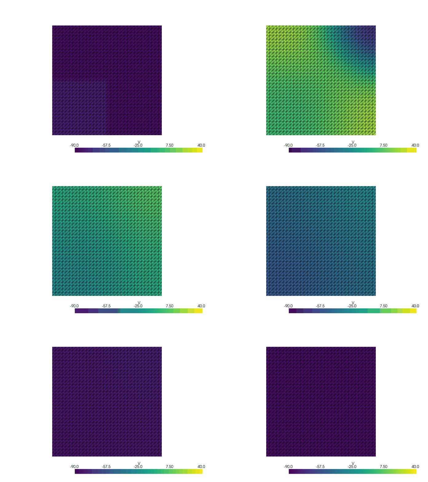
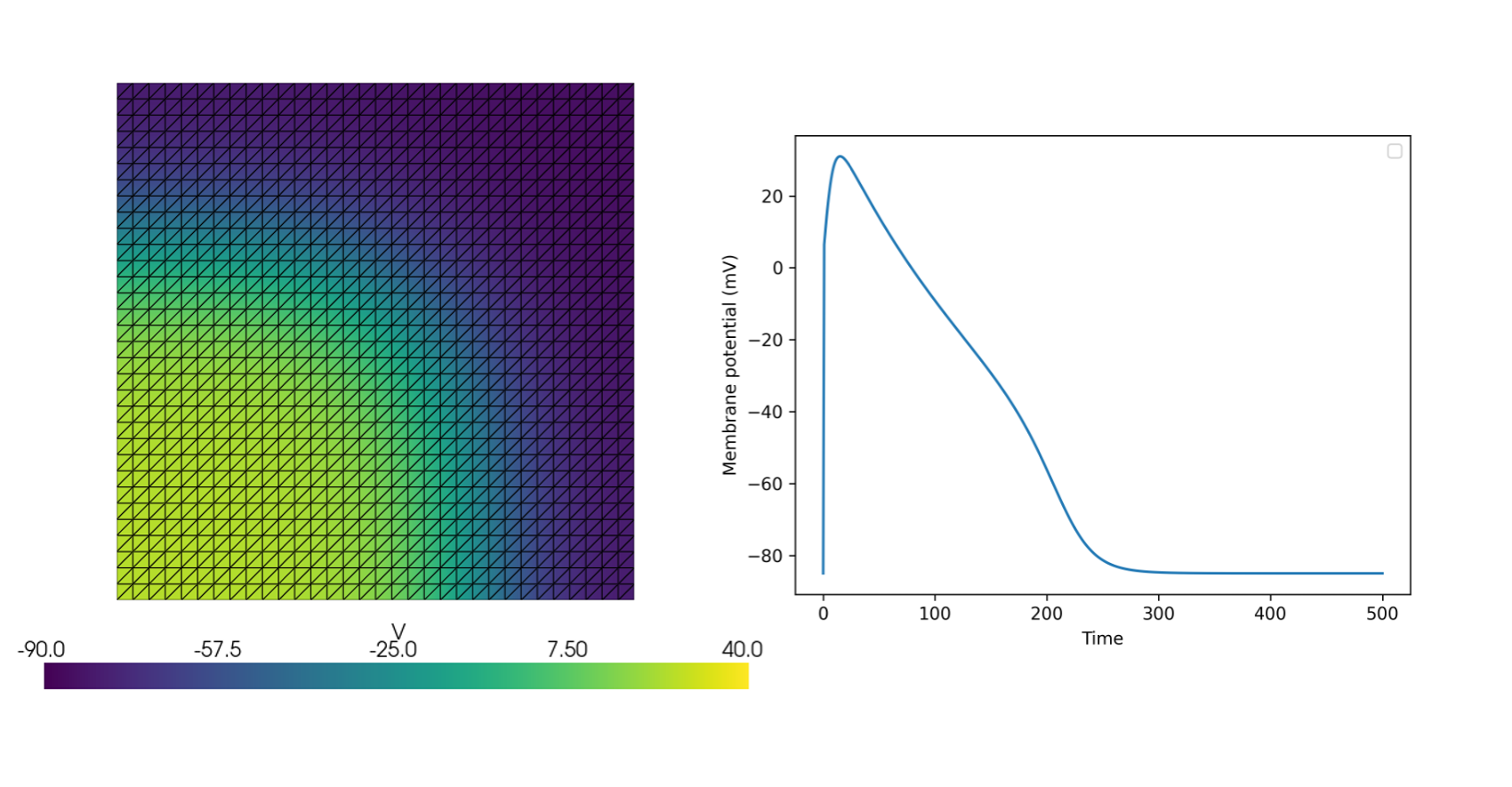
The following minimal example demonstrates simulating the Monodomain model on a unit square domain using a modified FitzHugh-Nagumo model
import shutil

import matplotlib.pyplot as plt
import numpy as np

from mpi4py import MPI
import dolfinx
import ufl

import beat

# MPI communicator
comm = MPI.COMM_WORLD
# Create mesh
mesh = dolfinx.mesh.create_unit_square(comm, 32, 32, dolfinx.cpp.mesh.CellType.triangle)
# Create a variable for time
time = dolfinx.fem.Constant(mesh, dolfinx.default_scalar_type(0.0))


# Define forward euler scheme for solving the ODEs
# This just needs to be a function that takes the current time, states, parameters and dt
# and returns the new states
def fitzhughnagumo_forward_euler(t, states, parameters, dt):
    s, v = states
    (
        c_1,
        c_2,
        c_3,
        a,
        b,
        v_amp,
        v_rest,
        v_peak,
        stim_amplitude,
        stim_duration,
        stim_start,
    ) = parameters
    i_app = np.where(
        np.logical_and(t > stim_start, t < stim_start + stim_duration),
        stim_amplitude,
        0,
    )
    values = np.zeros_like(states)

    ds_dt = b * (-c_3 * s + (v - v_rest))
    values[0] = ds_dt * dt + s

    v_th = v_amp * a + v_rest
    I = -s * (c_2 / v_amp) * (v - v_rest) + (
        ((c_1 / v_amp**2) * (v - v_rest)) * (v - v_th)
    ) * (-v + v_peak)
    dV_dt = I + i_app
    values[1] = v + dV_dt * dt
    return values


# Define space for the ODEs
ode_space = dolfinx.fem.functionspace(mesh, ("P", 1))

# Define parameters for the ODEs
a = 0.13
b = 0.013
c1 = 0.26
c2 = 0.1
c3 = 1.0
v_peak = 40.0
v_rest = -85.0
stim_amplitude = 100.0
stim_duration = 1
stim_start = 0.0

# Collect the parameter in a numpy array
parameters = np.array(
    [
        c1,
        c2,
        c3,
        a,
        b,
        v_peak - v_rest,
        v_rest,
        v_peak,
        stim_amplitude,
        stim_duration,
        stim_start,
    ],
    dtype=np.float64,
)

# Define the initial states
init_states = np.array([0.0, -85], dtype=np.float64)
# Specify the index of state for the membrane potential
# which will also inform the PDE solver later
v_index = 1

# We can also check the solution of the ODE
# by solving the ODE for a single cell
times = np.arange(0.0, 1000.0, 0.1)
values = np.zeros((len(times), 2))
values[0, :] = np.array([0.0, -85.0])
for i, t in enumerate(times[1:]):
    values[i + 1, :] = fitzhughnagumo_forward_euler(t, values[i, :], parameters, dt=0.1)


fig, ax = plt.subplots()
ax.plot(times, values[:, v_index])
ax.set_xlabel("Time")
ax.set_ylabel("States")
ax.legend()
fig.savefig("ode_solution.png")


# Now we set external stimulus to zero for ODE
parameters[-3] = 0.0

# and create stimulus for PDE
stim_expr = ufl.conditional(ufl.And(ufl.ge(time, 0.0), ufl.le(time, 0.5)), 600.0, 0.0)
stim_marker = 1
cells = dolfinx.mesh.locate_entities(
    mesh, mesh.topology.dim, lambda x: np.logical_and(x[0] <= 0.5, x[1] <= 0.5)
)
stim_tags = dolfinx.mesh.meshtags(
    mesh,
    mesh.topology.dim,
    cells,
    np.full(len(cells), stim_marker, dtype=np.int32),
)
dx = ufl.Measure("dx", domain=mesh, subdomain_data=stim_tags)
I_s = beat.Stimulus(expr=stim_expr, dZ=dx, marker=stim_marker)

# Create PDE model
pde = beat.MonodomainModel(time=time, mesh=mesh, M=0.001, I_s=I_s, dx=dx)

# Next we create the PDE solver where we make sure to
# pass the variable for the membrane potential from the PDE
ode = beat.odesolver.DolfinODESolver(
    v_ode=dolfinx.fem.Function(ode_space),
    v_pde=pde.state,
    fun=fitzhughnagumo_forward_euler,
    init_states=init_states,
    parameters=parameters,
    num_states=len(init_states),
    v_index=1,
)

# Combine PDE and ODE solver
solver = beat.MonodomainSplittingSolver(pde=pde, ode=ode)

# Now we setup file for saving results
# First remove any existing files
shutil.rmtree("voltage.bp", ignore_errors=True)

vtx = dolfinx.io.VTXWriter(mesh.comm, "voltage.bp", [pde.state], engine="BP5")
vtx.write(0.0)

# Finally we run the simulation for 400 ms using a time step of 0.01 ms
T = 400.0
t = 0.0
dt = 0.01
i = 0
while t < T:
    v = solver.pde.state.x.array
    solver.step((t, t + dt))
    t += dt
    if i % 500 == 0:
        vtx.write(t)
    i += 1

vtx.close()
See more examples in the documentation
Citation
If you use this software in your research, please cite the following paper
@article{Finsberg2025,
    doi = {10.21105/joss.08416},
    url = {https://doi.org/10.21105/joss.08416},
    year = {2025},
    publisher = {The Open Journal},
    volume = {10},
    number = {114},
    pages = {8416},
    author = {Finsberg, Henrik},
    title = {fenicsx-beat - An Open Source Simulation Framework for Cardiac Electrophysiology},
    journal = {Journal of Open Source Software}
}
License
MIT
Need help or having issues
Please submit an issue
1 maintainer

Release files for fenicsx-beat 0.6.0
For a detailed explanation of source distributions (sdists) and built distributions (wheels), please see the package formats documentation.
Source distribution (sdist)
| File | Size | Uploaded | |
|---|---|---|---|
| fenicsx_beat-0.6.0.tar.gz | 57.4 kB | Details |
Built distribution (wheel)
| File | Interpreter | ABI | Platform | Reset |
|---|---|---|---|---|
| fenicsx_beat-0.6.0-py3-none-any.whl | Python 3 | none | any | Details |
Total release size: 102.4 kB
Release files / fenicsx_beat-0.6.0.tar.gz
| Download URL | fenicsx_beat-0.6.0.tar.gz |
|---|---|
| Size | 57.4 kB |
| Tags | Source |
|
SHA-256 checksum How to use checksums |
e66011c5664af0c186f8ebc5aa5bad9f5b07cc1bddd481df9bc00da389a30860
|
|
BLAKE2b-256 checksum How to use checksums |
8d51e7ff131f3f8811dcd927d6425bdcdd62b5a9d3833824b2cfd9f3dac09fc7
|
| Upload date | |
|
Uploaded using Trusted Publishing? What is trusted publishing? |
Yes |
| Uploaded via |
twine/7.0.0 CPython/3.13.14
|
Provenance
Provenance describes where a file came from. On PyPI, provenance is shared via attestations, which provide a verifiable record of the build or publishing details. View details, limitations and caveats.


PyPI Publish Attestation
PyPI verified that this artifact, at this checksum, originated from the publisher listed below.
Signed by GitHub Actions, verified by PyPI on Sep 22, 2026.
Transparency logRelease files / fenicsx_beat-0.6.0-py3-none-any.whl
| Download URL | fenicsx_beat-0.6.0-py3-none-any.whl |
|---|---|
| Size | 45.1 kB |
| Tags | Python 3 |
|
SHA-256 checksum How to use checksums |
9b990cee02f69617eaea0448b2b072c57f23367f08ba5fd8b2b1faa4c6bebb99
|
|
BLAKE2b-256 checksum How to use checksums |
5a8067c11eb049441da59e366391aba9c8df1019d46d4747bd37384bd791b08d
|
| Upload date | |
|
Uploaded using Trusted Publishing? What is trusted publishing? |
Yes |
| Uploaded via |
twine/7.0.0 CPython/3.13.14
|
Provenance
Provenance describes where a file came from. On PyPI, provenance is shared via attestations, which provide a verifiable record of the build or publishing details. View details, limitations and caveats.
PyPI Publish Attestation
PyPI verified that this artifact, at this checksum, originated from the publisher listed below.
Signed by GitHub Actions, verified by PyPI on Sep 22, 2026.
Transparency log













