FFT-based contrast-to-noise ratio estimation from a single frame
Verified details
These details have been verified by PyPIProject links
GitHub Statistics
Maintainers

Project description
fft-cnr


FFT-based contrast-to-noise ratio estimation from a single frame.
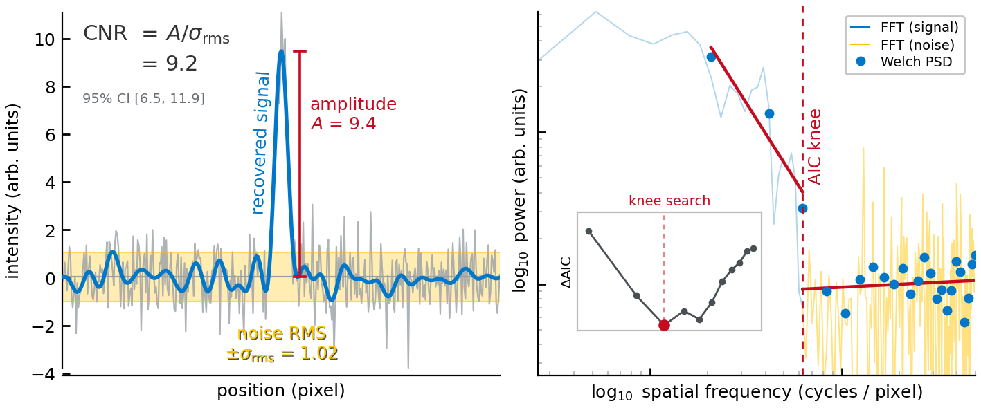
Measure the contrast-to-noise ratio (CNR) of a 1-D signal profile from a single acquisition. You do not need repeat frames or a separate background region.
Here CNR means the peak signal amplitude above the baseline, divided by the RMS of the noise. This is a peak-amplitude signal-to-noise ratio, not a two-region (difference-of-means) contrast measure.
fft-cnr uses the Fourier transform to separate the slowly varying signal from
the rapid, point-to-point noise. The package automatically finds the frequency
boundary between the two (using a model-selection score, the Akaike information
criterion or AIC) and returns a CNR estimate with a 95% confidence interval.
Installation
Requires Python 3.10 or later (tested on 3.10 through 3.13). If you do not have Python installed, download it from python.org and follow the installer instructions (on Windows, check "Add Python to PATH" when prompted).
Install into a virtual environment so the package and its dependencies stay isolated from your other projects:
python -m venv .venv
source .venv/bin/activate   # Windows: .venv\Scripts\activate
pip install fft-cnr
The only runtime dependencies are numpy (>=1.24) and scipy (>=1.10); pip installs them automatically.
Quick start
import numpy as np
from fft_cnr import fft_cnr

# Simulate a 1-D intensity profile (e.g., from a microscopy line scan)
# with additive detector noise
rng = np.random.default_rng(0)
x = np.arange(256, dtype=float)
signal = 10.0 * np.exp(-0.5 * ((x - 127) / 20) ** 2)
noisy = signal + rng.normal(0, 1.0, 256)

result = fft_cnr(noisy)

print(f"CNR:       {result.cnr:.1f}")
print(f"CNR 95%CI: ({result.cnr_ci95[0]:.1f}, {result.cnr_ci95[1]:.1f})")
print(f"Amplitude: {result.amplitude:.2f}")
print(f"Noise RMS: {result.noise_rms:.3f}")
CNR:       9.8
CNR 95%CI: (6.9, 12.7)
Amplitude: 9.74
Noise RMS: 0.991
The output is deterministic given the seed, so this snippet reproduces the same
numbers on each run. The package exposes three names: the fft_cnr function and
its result types CNREstimate and NoiseModel.
How it works
A smooth signal spread over many points concentrates its energy in a few low-frequency Fourier components. Uncorrelated, point-to-point noise spreads its energy across all frequencies. So in the power spectrum the signal sits at low frequency and the noise dominates the high-frequency end, which is where the two can be separated.
- The input profile is mean-subtracted and tapered with a window function (a tapered cosine, or Tukey, window by default) to suppress edge artifacts in the Fourier transform.
- The power spectrum is estimated by averaging the transforms of overlapping segments, which is smoother than a single transform (the averaged-segment, or Welch, method). More segments give the noise estimate more degrees of freedom, which tightens its confidence interval; this does not by itself improve the CNR point estimate.
- The power spectrum typically shows high power at low frequencies, where the signal lives, that levels off to a flat noise floor at higher frequencies. The algorithm finds this transition by fitting two line segments in log-log space. It then uses the Akaike information criterion (AIC, a standard score that penalizes overfitting) to pick the boundary that best balances fit quality against model complexity.
- The spectral bins at and below the boundary are set to zero, the remaining high-frequency bins are transformed back to real space, and the RMS of that reconstructed noise is taken. This RMS is then scaled to undo the window energy and the fraction of bins kept, so it estimates the full-band noise level.
- Signal amplitude is estimated by one of three methods (see below), and CNR = amplitude / noise RMS.
- A 95% confidence interval on CNR is computed by first-order error propagation (the delta method), combining the amplitude error and the chi-squared noise interval.
The method works best when the signal occupies low frequencies and the noise is
broadband (approximately white). The hard minimum length is 16 points (shorter
inputs raise ValueError); reliable knee detection needs more, with measurable
bias below roughly 128 points (see Accuracy). Signals with strong high-frequency
content that overlaps the noise band will also bias the CNR estimate.
Amplitude estimation
By default (fit_model=None or "peak"), fft_cnr removes the high-frequency
noise components (by zeroing frequencies above the signal/noise boundary) and
reads the peak of the resulting smoothed profile, measured above a baseline
estimated from the outer quarter of the profile on each side. This works for any
profile shape and assumes nothing about its functional form. If the signal
extends into those outer regions, the baseline is contaminated and the amplitude
is underestimated.
Two alternatives are available:
-
Matched filter (
templateparameter): when a noise-free template of the expected signal shape is available, a matched filter gives the most precise amplitude estimate and a calibrated standard error. This holds only when the template matches the true shape; a mismatched template biases the amplitude. -
Generalized Gaussian fit (
fit_model="generalized_gaussian"): fits a 5-parameter model with a shape exponent that covers profiles from heavy-tailed to flat-topped. Useful when fitted parameters (center, width, shape) are needed in addition to CNR.
The result.amplitude_snr property reports the matched-filter signal-to-noise
ratio (amplitude over its standard error). A larger value means the amplitude
stands out more clearly above the noise. It is defined only on the matched-filter
(template) path, where the standard error is calibrated; on the peak and
generalized-Gaussian paths it is NaN, because those standard errors are
different quantities that are not comparable to it. Those paths still expose
amplitude_se directly for callers that want the raw ratio.
# With a known template
result = fft_cnr(noisy, template=signal)

# With a generalized Gaussian fit
result = fft_cnr(noisy, fit_model="generalized_gaussian")
print(result.diagnostics["gaussian_fit_params"])
Noise model detection
The CNR above treats the noise as one number, which is correct when the noise
is the same at every point (for example, detector read noise). Photon-counting
measurements break this assumption. Shot noise grows with the local signal, so
the noise under the peak is larger than the average noise. Because cnr divides
the peak by the average noise, it overestimates the true peak signal-to-noise
ratio, and the size of the error depends on the profile shape.
Setting estimate_noise_model=True makes fft_cnr test for this. It fits the
photon-transfer relation (variance = gain * signal + read^2) to its own
residual, a single-frame surrogate for a photon-transfer curve that is
conventionally measured from many exposures, and attaches a NoiseModel to the
result:
result = fft_cnr(noisy, estimate_noise_model=True)
model = result.noise_model

if model.signal_dependent:
    # Noise grows with the signal; result.cnr overestimates the peak SNR.
    # The fitted noise model gives the corrected value:
    print(f"Peak SNR: {model.peak_snr(result.amplitude):.1f}")
model.signal_dependent is True when the fitted gain is statistically
significant, False when the noise is consistent with a constant level, and
None when the profile's signal range is too small to test (the reason
appears in diagnostics["noise_model_skipped"]). To judge significance, the
package runs the whole estimation pipeline on about 200 simulated data sets, so
the test accounts for the estimator's own artifacts. These extra runs cost
roughly half a second at N=512.
The detection is deterministic by default: the same input always produces the
same result. Pass your own random generator (rng=np.random.default_rng())
to draw an independent simulation instead.
Estimating a Poisson-Gaussian noise model from a single image is established prior art, most notably the single-image method of Foi et al. (IEEE Trans. Image Process. 17, 1737 (2008)). This detector does not claim to be first at single-frame noise estimation. What it adds is to fold the photon-transfer fit into the spectral decomposition the CNR already computes, gated by a significance test calibrated through the same pipeline.
Correlated (1/f) noise is not corrected
Signal-dependence is one way the constant-noise assumption fails. Spatially
correlated, 1/f-type noise is a separate one. It arises when temporal drift maps
onto a spatial direction, as in galvo raster scanning or streak cameras. The
drift puts noise power at low spatial frequency, where fft_cnr reads signal,
so it biases cnr high.
The NoiseModel has fields for this case (spectral_exponent, white_floor,
and correlated), but they are reserved and not filled in: the two floats stay
NaN and the flag stays None. Single-frame quantitative correction of correlated
noise is not supported, and the reason is an identifiability limit. The signal
and the 1/f noise both live in the low frequencies, and a single profile gives
one measurement, so there is no way to tell how much of the low-frequency power
is signal and how much is drift; any split fits the data equally well.
Separating them needs a second, independent view in which the signal repeats but
the noise does not: multiple frames, an interleaved scan, or a reference
channel. Those are also the way to correct correlated noise once it is detected.
Low-frequency baseline and structured background
A smooth baseline, a slow trend or a single low-frequency fringe, sits entirely
below the signal/noise boundary, so fft_cnr reads it as signal. With a strong
baseline the peak-method cnr can stay high even for a profile with no peak.
Two tools address this:
diagnostics["lowfreq_dominated"](with the underlyinglowfreq_offpeak_ratio) is true when low-frequency structure away from the peak exceeds 2.5 times the noise RMS. It marks profiles where the reportedcnrmay reflect baseline power rather than the peak. The flag is set on the peak and generalized-Gaussian methods and is not set on the matched-filter path, where the template defines the signal.roirestricts the estimate to a window around the peak, removing off-center baseline structure. Pass explicit(start, stop)bounds, or"auto"to size a window to the peak."auto"locates the largest feature, so pass explicit bounds when an off-center baseline is larger than the peak of interest.
This guard is calibrated for smooth, low-order baselines. Broadband structured
background is a different problem. The residual speckle and fringe field left
after interferometric scattering microscopy (iSCAT) background subtraction is
the representative case: its power spans many spatial frequencies, including the
high-frequency band that sets the noise estimate. It both inflates the noise
RMS, which suppresses real peaks, and adds low-frequency amplitude, which raises
peakless frames, so the peak-method cnr is unreliable and lowfreq_dominated
does not detect it. This is correlated noise (see above) and cannot be
characterized from a single frame.
For this regime, use the matched filter: pass the known signal shape as
template and read amplitude and amplitude_snr rather than cnr. The
projection onto the template rejects background that does not match the template
shape, so the amplitude and its SNR stay accurate where cnr does not. For
iSCAT the template is the interferometric point-spread function. The
scripts/validate_iscat_baseline.py simulation documents this behavior.
Return value
fft_cnr returns a CNREstimate dataclass. The first five fields are the
primary outputs; cutoff_index, diagnostics, and noise_model are for
advanced inspection.
| Field | Type | Description |
|---|---|---|
cnr |
float |
Estimated contrast-to-noise ratio |
cnr_ci95 |
tuple[float, float] |
95% confidence interval on CNR |
amplitude |
float |
Signal amplitude estimate (signed on the peak path: negative for a dip) |
amplitude_se |
float |
Standard error of the amplitude estimate |
amplitude_snr |
float (property) |
Matched-filter SNR (amplitude over its standard error); NaN on the peak and generalized-Gaussian paths |
noise_rms |
float |
RMS noise from the high-frequency spectral region |
noise_ci95 |
tuple[float, float] |
95% confidence interval on noise RMS |
cutoff_index |
int |
Spectral index of the signal/noise boundary |
diagnostics |
dict |
Welch parameters, DOF, amplitude method, fit params, low-frequency baseline guard (lowfreq_dominated, lowfreq_offpeak_ratio), peak-read sign-ambiguity flag (amplitude_sign_ambiguous), and roi bounds when set |
noise_model |
NoiseModel | None |
Fitted noise structure (None unless requested) |
Parameters
Most users will only need x (and optionally template or fit_model). The
remaining parameters control internal details of the spectral estimation and
rarely need adjustment.
| Parameter | Default | Description |
|---|---|---|
x |
(required) | 1-D signal array (length >= 16) |
template |
None |
Noise-free template for matched-filter estimation |
fit_model |
None |
Amplitude method: None/"peak" for spectral low-pass, "generalized_gaussian" for parametric fit |
window |
"tukey" |
Taper window: "tukey", "hann", or "none" |
tukey_alpha |
0.25 |
Tukey window shape parameter |
welch_nperseg |
None |
Welch segment length (defaults to max(16, N//8)) |
welch_noverlap |
None |
Welch overlap (defaults to nperseg // 2) |
cutoff_guard |
(0.05, 0.5) |
Fractional frequency bounds for signal/noise boundary search |
fallback_cut_frac |
0.25 |
Fallback signal/noise boundary if AIC selection fails |
roi |
None |
Restrict to a region of interest: (start, stop) bounds or "auto" (see Low-frequency baseline and structured background) |
return_bandpassed_noise |
False |
Include the bandpassed noise array in diagnostics |
estimate_noise_model |
False |
Fit and test the noise model (see Noise model detection) |
rng |
None |
Generator for the noise-model test; None is deterministic |
The minimum accepted length is 16 points. Reliable results need more; see How it works for guidance on length.
Accuracy
Monte Carlo validation (200 trials per condition, scripts/validate_accuracy.py)
characterizes bias, precision, and confidence-interval coverage across five
signal shapes: Gaussian, heavy-tailed (generalized Gaussian, p=1.5),
flat-topped (p=4), Gaussian mixture, and Lorentzian. All conditions use additive
white Gaussian noise, the regime the method assumes, so the headline accuracy
numbers inherit that assumption.
Bias
Median estimated-to-true CNR ratio at N=512, by amplitude method:
| Shape | Peak | Gen. Gaussian | Matched filter |
|---|---|---|---|
| Gaussian | 1.00--1.03 | 1.00--1.01 | 1.00--1.01 |
| Heavy-tailed (p=1.5) | 0.97--1.00 | 0.99--1.01 | 0.98--1.00 |
| Flat-topped (p=4) | 0.93--1.10 | 0.93--1.01 | 0.92--1.00 |
| Gaussian mixture | 0.99--1.01 | 1.12--1.16 | 0.99--1.00 |
| Lorentzian | 0.98--1.01 | 1.06--1.09 | 0.99--1.00 |
The peak method stays within 3% of the true CNR for most shapes from CNR=5 upward. The main exception is flat-topped profiles, where the spectral low-pass filter rounds off the flat peak (up to 7% positive bias at CNR=3, 7% negative at CNR=100). The generalized Gaussian fit is accurate when the signal is in the model family but introduces 6--16% positive bias on shapes outside it (Gaussian mixture, Lorentzian). The matched filter tracks the true CNR to within 2% when the template matches the signal shape.
Profile length
Shorter profiles reduce accuracy slightly. At N=128 (peak method, Gaussian signal), the estimator shows 6--8% negative bias at high CNR because the Welch PSD has fewer segments for knee detection.
| N | CNR=5 | CNR=20 | CNR=100 |
|---|---|---|---|
| 128 | 1.03 | 0.94 | 0.93 |
| 256 | 1.03 | 1.00 | 1.00 |
| 512 | 1.01 | 1.01 | 1.00 |
Precision
Trial-to-trial scatter (relative standard deviation) scales as roughly 1/sqrt(N): approximately 11% at N=128, 7% at N=256, and 5% at N=512 (peak method, CNR=5). Providing a matched template reduces scatter at low CNR.
Confidence intervals
The 95% confidence intervals contain the true value in 99 to 100% of trials across all tested conditions, so they are reliable but wider than a true 95% interval. The interval combines two terms, the uncertainty in the amplitude and the uncertainty in the noise level, and which term makes it wide depends on the amplitude method.
For the peak and generalized-Gaussian methods the noise term dominates. The degrees of freedom used for the chi-squared noise interval are set conservatively, so that term, and the combined interval, come out wider than nominal.
For the matched-filter method (a supplied template) the amplitude standard error is the exact closed-form error of the white-noise projection: the windowed data projected onto the windowed template, with error sigma divided by the template norm for a flat window. The noise term still dominates the combined interval at the conservative degrees of freedom above, so the matched-filter interval comes out comparable in width to the others while resting on the most precise amplitude estimate.
Noise model detection
Monte Carlo validation of the signal-dependence test (100 trials per
condition, scripts/validate_noise_model.py) covers white noise, where the
test should stay quiet, and Poisson counts, where it should fire. Conditions
span Gaussian and flat-topped profiles, N in {256, 512}, and CNR 5--20; no
trial was skipped for insufficient signal range.
| Regime | Flag rate | Median gain | Median read |
|---|---|---|---|
| White noise (truth: gain 0, read 1) | 2--7% (nominal 5%) | -0.004 to +0.007 | 0.99--1.00 |
| Poisson counts (truth: gain 1, read 0) | 100% | 0.95--1.02 | -- |
On white noise the false-positive rate is consistent with the 5% test level and the fitted parameters recover the truth. On Poisson data the test fired in all 100 trials at these conditions, the fitted gain is within 5% of the true value, and the derived peak SNR tracks the true peak signal-to-noise ratio (ratio 0.99 to 1.03 across N and CNR).
Citation
If you use fft-cnr in published work, please cite it. The concept DOI below
always resolves to the latest release; to cite the exact version you used, take
that version's DOI from the Zenodo record and report the pinned version
(pip install fft-cnr==0.3.0).
Joseph J. Thiebes. fft-cnr: FFT-based contrast-to-noise ratio estimation from a single frame. Zenodo. https://doi.org/10.5281/zenodo.20691435
@software{thiebes_fft_cnr,
  author    = {Thiebes, Joseph J.},
  title     = {fft-cnr: FFT-based contrast-to-noise ratio estimation from a single frame},
  version   = {0.3.0},
  year      = {2026},
  publisher = {Zenodo},
  doi       = {10.5281/zenodo.20691435},
  url       = {https://doi.org/10.5281/zenodo.20691435}
}
Citation metadata is in CITATION.cff; GitHub's "Cite this repository" button generates APA and BibTeX from it.
Background
The spectral decomposition approach used here originated in a study of noise effects on diffusion coefficient estimation in chemical transport imaging (Thiebes & Grumstrup, 2024). This package has evolved from the method described in that paper. The power-spectrum estimation, knee detection, and confidence-interval machinery all differ from the original.
Support for non-Gaussian profiles was motivated by work on excess kurtosis in exciton transport (Arévalo Rodríguez et al., 2026).
Methods and background. The package implements established signal-processing and sensor-characterization methods: averaged-periodogram power-spectrum estimation (Welch, 1967), window tapering for harmonic analysis (Harris, 1978), model selection by the Akaike information criterion (Akaike, 1974), matched filtering (North, 1963; Turin, 1960), the estimation-theory framework for standard errors and the Cramér-Rao bound on estimator variance (Kay, 1993), and the photon-transfer characterization of sensor noise (Janesick, 2007; EMVA Standard 1288). Estimating a Poisson-Gaussian noise model from a single image is established separately (Foi et al., 2008); this package folds a photon-transfer fit into the spectral decomposition it already computes rather than reimplementing that method. Full references with DOIs are listed under References below; machine-readable citation metadata is in CITATION.cff.
References
- Akaike, H. (1974). A new look at the statistical model identification. IEEE Transactions on Automatic Control, 19(6), 716-723. doi:10.1109/TAC.1974.1100705
- Arévalo Rodríguez, E., Meléndez, M., Cuadra, J., & Prins, F. (2026). Journal of Physical Chemistry Letters, 17, 2479-2484. doi:10.1021/acs.jpclett.5c03961
- European Machine Vision Association (2021). EMVA Standard 1288: Standard for Characterization of Image Sensors and Cameras, version 4.0. emva.org
- Foi, A., Trimeche, M., Katkovnik, V., & Egiazarian, K. (2008). Practical Poissonian-Gaussian noise modeling and fitting for single-image raw-data. IEEE Transactions on Image Processing, 17(10), 1737-1754. doi:10.1109/TIP.2008.2001399
- Harris, F. J. (1978). On the use of windows for harmonic analysis with the discrete Fourier transform. Proceedings of the IEEE, 66(1), 51-83. doi:10.1109/PROC.1978.10837
- Janesick, J. R. (2007). Photon Transfer. SPIE Press. doi:10.1117/3.725073
- Kay, S. M. (1993). Fundamentals of Statistical Signal Processing, Volume I: Estimation Theory. Prentice Hall. ISBN 978-0-13-345711-7.
- North, D. O. (1963). An analysis of the factors which determine signal/noise discrimination in pulsed-carrier systems. Proceedings of the IEEE, 51(7), 1016-1027. doi:10.1109/PROC.1963.2383
- Thiebes, J. J., & Grumstrup, E. M. (2024). Journal of Chemical Physics, 160, 124201. doi:10.1063/5.0190347
- Turin, G. L. (1960). An introduction to matched filters. IRE Transactions on Information Theory, 6(3), 311-329. doi:10.1109/TIT.1960.1057571
- Welch, P. D. (1967). The use of fast Fourier transform for the estimation of power spectra: A method based on time averaging over short, modified periodograms. IEEE Transactions on Audio and Electroacoustics, 15(2), 70-73. doi:10.1109/TAU.1967.1161901
Acknowledgments
Thanks to Ferry Prins and Enrique Arévalo Rodríguez for discussions on non-Gaussian transport profiles that informed the design of this package.
Contributing and community
Contributions, bug reports, and feature requests are welcome. See CONTRIBUTING.md for development setup, how to run the tests, and how to submit changes. Participation is governed by the Code of Conduct.
Development disclosure
The method, design, and direction of this package are the author's own. It builds on the author's prior work: the spectral contrast-to-noise estimator introduced in Thiebes and Grumstrup (2024) and developed further in the DICE repository (see Background). The estimator's structure, the choices behind each pipeline step, the validation strategy, and the critique that shaped successive revisions all reflect the author's own thinking.
Generative AI tools (Anthropic Claude) assisted primarily with code: drafting implementations from the author's specifications, writing tests, and editing documentation. The author directed this work, reviewed and corrected every contribution, and characterized the estimator by the Monte Carlo validation reported under Accuracy.
License
Released under the MIT License; see the LICENSE file for the full text.
Project details
Verified details
These details have been verified by PyPIProject links
GitHub Statistics
Maintainers


Download files
Download the file for your platform. If you're not sure which to choose, learn more about installing packages.
Source Distribution
Built Distribution
Filter files by name, interpreter, ABI, and platform.
If you're not sure about the file name format, learn more about wheel file names.
Copy a direct link to the current filters
File details
Details for the file fft_cnr-0.3.0.tar.gz.
File metadata
- Download URL: fft_cnr-0.3.0.tar.gz
- Upload date:
- Size: 394.2 kB
- Tags: Source
- Uploaded using Trusted Publishing? Yes
- Uploaded via: twine/6.1.0 CPython/3.13.13
File hashes
| Algorithm | Hash digest | |
|---|---|---|
| SHA256 |
358c28999a10e8a9d16e83a6adc259bdc8930e570076987959d17248177faa43
|
|
| MD5 |
2dfe49b1ed6b3734d7f2e17bf689dcbb
|
|
| BLAKE2b-256 |
3ce7f6b5e95bb0b2ebf0943e1485c9fbc61861f7042eb9463eb3acc561e27c09
|
Provenance
The following attestation bundles were made for fft_cnr-0.3.0.tar.gz:
Publisher:
publish.yml on thiebes/fft-cnr
-
Statement:
-
Statement type:
https://in-toto.io/Statement/v1 -
Predicate type:
https://docs.pypi.org/attestations/publish/v1 -
Subject name:
fft_cnr-0.3.0.tar.gz -
Subject digest:
358c28999a10e8a9d16e83a6adc259bdc8930e570076987959d17248177faa43 - Sigstore transparency entry: 2000462166
- Sigstore integration time:
-
Permalink:
thiebes/fft-cnr@e898f262a1807fead5da4f9af07ff0151c9add92 -
Branch / Tag:
refs/tags/v0.3.0 - Owner: https://github.com/thiebes
-
Access:
public
-
Token Issuer:
https://token.actions.githubusercontent.com -
Runner Environment:
github-hosted -
Publication workflow:
publish.yml@e898f262a1807fead5da4f9af07ff0151c9add92 -
Trigger Event:
release
-
Statement type:
File details
Details for the file fft_cnr-0.3.0-py3-none-any.whl.
File metadata
- Download URL: fft_cnr-0.3.0-py3-none-any.whl
- Upload date:
- Size: 24.7 kB
- Tags: Python 3
- Uploaded using Trusted Publishing? Yes
- Uploaded via: twine/6.1.0 CPython/3.13.13
File hashes
| Algorithm | Hash digest | |
|---|---|---|
| SHA256 |
5ec0922e584ea8071506101b2d285378ac037d8bd767a589125d4f50976b90a8
|
|
| MD5 |
bac6efaf7bdae51faf87628d0088f124
|
|
| BLAKE2b-256 |
4d8c72eb617e1f831f00507b52052f80400ecd779fbb583fb853ac45b3e5682b
|
Provenance
The following attestation bundles were made for fft_cnr-0.3.0-py3-none-any.whl:
Publisher:
publish.yml on thiebes/fft-cnr
-
Statement:
-
Statement type:
https://in-toto.io/Statement/v1 -
Predicate type:
https://docs.pypi.org/attestations/publish/v1 -
Subject name:
fft_cnr-0.3.0-py3-none-any.whl -
Subject digest:
5ec0922e584ea8071506101b2d285378ac037d8bd767a589125d4f50976b90a8 - Sigstore transparency entry: 2000462221
- Sigstore integration time:
-
Permalink:
thiebes/fft-cnr@e898f262a1807fead5da4f9af07ff0151c9add92 -
Branch / Tag:
refs/tags/v0.3.0 - Owner: https://github.com/thiebes
-
Access:
public
-
Token Issuer:
https://token.actions.githubusercontent.com -
Runner Environment:
github-hosted -
Publication workflow:
publish.yml@e898f262a1807fead5da4f9af07ff0151c9add92 -
Trigger Event:
release
-
Statement type:


