
FiberNet + FiberScope
An open workflow for constructing, simulating, and studying fiber networks in Python and a desktop interface.
FiberNet supplies programmable graph, generation, analysis, and modeling tools. FiberScope is the interactive application built around fiber-network design workflows. Version 4.2.0 shares the core manufacturing, reduced simulation, physical learning, inverse-design, and recruitment calculations across Python and the APP. The published package and Windows desktop downloads are linked below; optional or experimental workflows are identified where they appear.
Start here · 3D generation · Planar generation · Stretch and recruitment · Machine learning · Optimization and RL · Python quick start · Desktop application · Methods · Current coverage
Start here
The library and desktop APP live in this existing fibernet repository. Install the 4.2.0 library with python -m pip install fibernet==4.2.0. Download the Windows APP from GitHub Releases; it does not require a local Python installation. The repository and release map describes the shared and APP-only features.
With Python 3.10, from the repository root, install the checkout with python -m pip install -e .. The complete runnable workflow uses the library's beam-frame FEM and does not require the desktop APP. The animated 3×3 kagome stretch below uses the shared reduced spring/bending/contact solver, also available without the APP through the trajectory example. These are different models with different assumptions.
| If you want to... | Start with | What you get |
|---|---|---|
| Generate or inspect a 2D network | pattern_2d, show |
A graph with nodes, edges, radii, and an optional figure |
| Stretch a small network in Python | simulate(..., backend="fem") |
Displacement, stress-related metadata, and a serializable result |
| Replay the APP's reduced stretch model in Python | ReducedBeamSolver, ReducedBeamConfig |
Node frames, edge strain, raw reaction, bending/contact energy |
| Analyze thresholded edge recruitment | analyze_tensile_recruitment |
Per-frame active edges, grip-spanning components, and threshold curves |
| Measure a planar network snapshot | SnapshotFeatureExtractor |
Structural, bounded-pore, distribution and optional finite-width contact descriptors |
| Study many generated networks | batch_simulate |
A CSV with measured force, displacement, and energy summaries |
| Build a closed planar or curved route | PlanarManufacturingConfig, compile_planar, compile_surface |
Reference/actual coordinates, parallel edges, and a closed Euler route |
| Save a custom unit shared with the desktop editor | CustomCell, CustomCellRegistry |
APP-compatible JSON, a reusable graph, and a compilable route |
| Create geometry files for inspection | build_solid, export_solid, export_route |
Closed mesh, STL/3MF, and edge-ordered CSV with optional dependencies |
| Use the visual manufacturing workspace | FiberScope desktop | Interactive configuration, path playback, and export tools |
The coverage audit states which advanced APP capabilities still need a public library API. The 4.2.0 wheel passed isolated Python 3.10 API checks, and source tests passed in 12 Linux/macOS/Windows and Python 3.9–3.12 CI combinations. Solver forces need calibration against experiment before quantitative material claims.
Explore three-dimensional networks
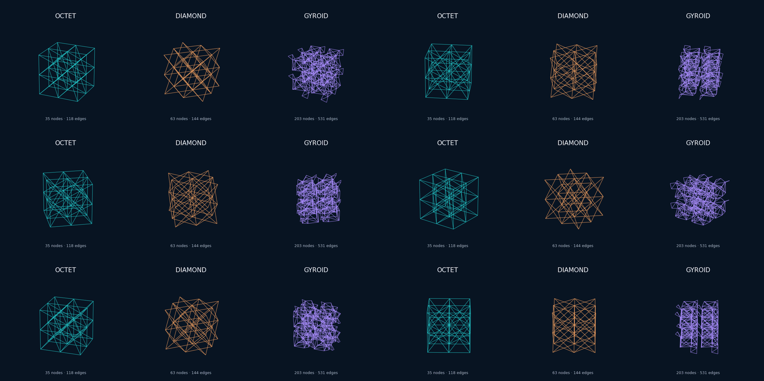
The library generates these three fixed 2×2×2 graphs with pattern_3d; only the camera rotates. Octet, diamond and gyroid have 35/118, 63/144 and 203/531 nodes/edges in this example. The editable vector keyframe, source and graph manifest, and python scripts/make_3d_homepage_media.py reproduce the gallery. Generate a network in Python with g = fibernet.pattern_3d(unit="gyroid", box=(2, 2, 2), grid=(2, 2, 2)); see the generation API for supported units. The APP's English 3D surface workspace maps fibers to OBJ surfaces and provides interactive inspection. A generated 3D graph is not a calibrated simulation or a printable toolpath.
Shape one profile across four topologies
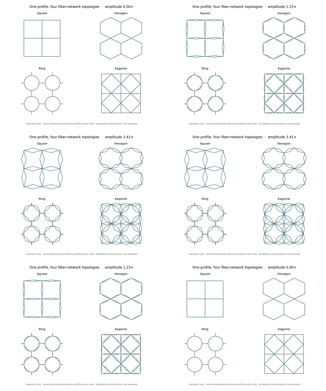
The square, hexagon, ring, and kagome panels use the same dimensionless reference-fiber displacement profile in the APP's current manufacturing-topology builder. The animation changes geometry while retaining each panel's graph connectivity. It is a geometry demonstration, not a printability or mechanical-performance result. The editable peak-frame SVG and source/parameter manifest accompany the GIF. Regenerate the spectrum and related animations with python scripts/make_homepage_media.py from the repository root. The profile and planar manufacturing builder are now shared through the Python library.
See the network respond
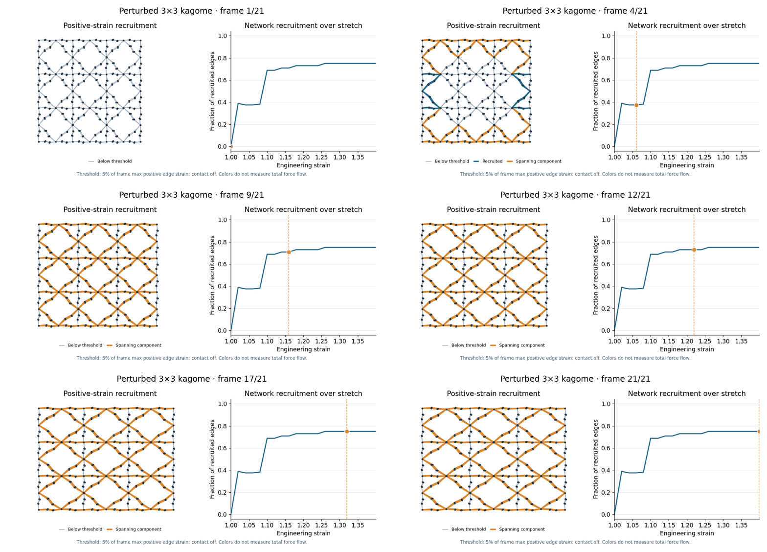
The perturbed 3×3 kagome network has 436 nodes and 576 edges and is stretched in the FiberScope reduced model. Blue edges exceed a positive-strain threshold; orange edges belong to a recruited component spanning both grips. The trace reports the fraction of recruited edges. These colors summarize a strain-threshold graph; they do not measure complete mechanical force flow. The animation and editable final-frame SVG have fixed parameters and a saved provenance/source-hash manifest.
Change the analysis threshold, keep the trajectory fixed
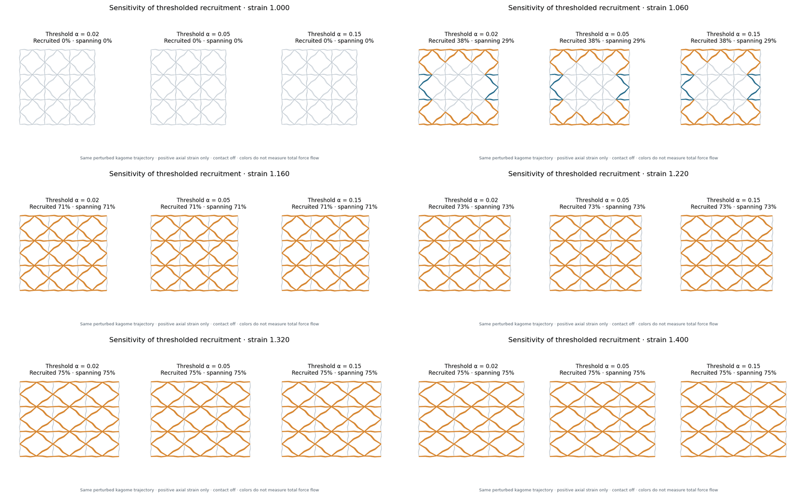
The three panels analyze the same node trajectories at α = 0.02, 0.05, and 0.15. Only the edge-strain threshold changes. The display makes parameter sensitivity visible before interpreting a connected path. Download the editable comparison SVG or inspect the parameter and source manifest. Neither the colors nor the thresholded connection prove local force transfer.
Compare loading directions on the same topology
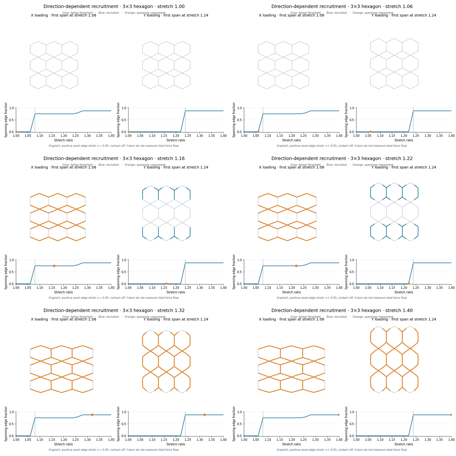
The same 3×3 hexagon topology is stretched horizontally and vertically. With a positive axial edge-strain minimum of 0.05, the reduced solver first finds a grip-spanning recruited component at stretch ratios 1.08 and 1.24, respectively. Gray edges remain below the threshold, blue edges are recruited, and orange edges belong to a spanning component. The editable vector keyframe and source/parameter manifest make this local example inspectable. This is a directional threshold statistic, not a full force-flow image; an independent nonlinear beam-FEM screen preserves the directional contrast at stretch 1.24 but does not reproduce the reduced solver's exact onset.
One model, two ways to work
| Task | Python library | FiberScope desktop |
|---|---|---|
| Basic 2D/3D patterns and graph operations | Available | Available |
| Thresholded tensile-strain recruitment | Public analysis API in 4.2.0 | Same shared calculation, visual playback |
| Reduced stretch/bending/contact solver | Public trajectory API and saved-array example | Same numeric core with interactive controls |
| Continuous planar/curved route, OBJ input and solid export | Public geometry APIs in 4.2.0 | Same shared geometry core plus interactive controls |
| Custom cell definitions and persistence | Shared bounded JSON registry and route compilation | Same registry core with visual editing |
| Physical labels, three-target surrogate and active sampling | Shared resumable label stream, six-model workflow and public 14-feature API | Same stream, model and acquisition core with data-generation UI |
| Target-curve inverse design | Shared curve/scalar objective search with a caller-supplied graph builder | Same search with interactive design controls |
| FEM and general ML tools | Available, with solver-specific assumptions | Selected workflows available |
| Structural, pore and finite-width contact snapshot cards | Shared bounded NumPy extractor; separate from the older 94-feature ML schema | Same calculation with interactive cards and region selection |
The capability audit lists the exact gaps and release gates. The APP's external RL trainer, AI assistant, and printer handoff are not equivalent pure-library workflows. Solver outputs require calibration before quantitative experimental prediction.
Python quick start
import numpy as np
from fibernet.analysis import analyze_tensile_recruitment

edges = np.array([[0, 1], [1, 2], [0, 2]])
edge_strain = np.array([[0.0, 0.0, 0.0], [0.2, 0.3, -0.1]])
result = analyze_tensile_recruitment(
    edge_strain, edges, left_nodes=[0], right_nodes=[2], n_nodes=3
)
print(result.perc_frame)  # 1
From a source checkout, run python -m examples.tensile_recruitment_quickstart for a complete executable example. The method definition documents thresholds, hysteresis, output fractions, and physical limits. The Python 3.10 test suite and an isolated installation of a locally built wheel have passed. Source tests also passed on Linux, macOS, and Windows with Python 3.9–3.12. Third-party-machine installation, frozen APP portability outside Windows, and broader optional-dependency combinations still need verification.
To replay the desktop APP's reduced model directly in Python, run python -m examples.reduced_recruitment_workflow --output-dir demo_stretch. The trajectory workflow saves node frames, ordered edges, edge axial strain, raw reaction, recruited masks, and a JSON summary. The solver includes axial springs, a degree-two bending approximation, and optional node contact; its method description distinguishes it from the beam-frame FEM below. Neither solver is calibrated to a material experiment here.
Generate, simulate, save, and analyze
Run python -m examples.open_source_workflow --output-dir demo_output from a source checkout. This executable Python 3.10 example creates a honeycomb graph, saves a network figure, runs a small-strain beam-frame FEM stretch, saves and reloads the simulation JSON, then calculates axial edge strain and thresholded grip-to-grip recruitment. The output directory contains network.png, fem_result.json, and summary.json. The small-strain FEM example is a software workflow check; its force is not calibrated to an experiment.
For direct use in a notebook:
import fibernet as fn

graph = fn.pattern_2d(unit="honeycomb", box=(10, 10), grid=(2, 2),
                      radius=0.05, seed=23)
result = fn.simulate(graph, backend="fem", mode="stretch", strain=1.01)
print(graph.num_nodes, graph.num_edges, result.max_displacement)
The full example shows edge ordering, grip selection, and result serialization explicitly. For several structures, fn.batch_simulate(configs, "results.csv", strain=1.01) writes max_force, max_displacement, and energy columns. In the beam-FEM backend, max_force is the largest individual beam axial force, computed with that beam's actual radius; it is not a grip reaction or an effective Young's modulus. energy is an axial-stress proxy rather than total bending-plus-contact energy. The public stretch shortcut retains independent parallel fibers; the beam-FEM API and units and corrected independent-model scope explain why those distinctions matter.
Measure a network snapshot
For the APP's structural, planar-pore and finite-width contact descriptors, run python -m examples.snapshot_features_workflow --output-dir demo_features --contact. The pure-library example writes scalar JSON and distribution NPZ; from fibernet.analysis import SnapshotFeatureExtractor, ContactConfig exposes the same calculation used by the APP's feature cards. Coordinates and contact width share a length unit, while pore/contact areas use its square. The feature definitions and budgets distinguish this snapshot schema from the library's older 94-feature ML extractor. Pixel overlap is a geometric descriptor, not contact force.
Train the shared physical surrogate
Install the optional ML dependencies with python -m pip install "fibernet[ml]==4.2.0" or python -m pip install -e ".[ml]" from source, then run python -m examples.physical_learning_workflow --output-dir demo_learning from a checkout. The runnable workflow defaults to clearly labeled synthetic data for checking the API; pass --data samples.npz with X shaped (N, 14) and physical Y shaped (N, 3) for your own peak, stiffness, and work labels. It writes held-out predictions and a metric summary. In Python, from fibernet.ml import light_features, PhysicalRegressor gives the same descriptor and six-model adapter used by FiberScope. The APP's English learning workspace exposes data generation, training and prediction. The method and leakage controls describe training-only normalization and the limits of a random holdout split. The synthetic demo is not evidence of material prediction accuracy.
Generate resumable physical labels
To create the physical-label dataset used for a later regressor, run python -m examples.physical_dataset_workflow --output-dir demo_labels --samples 8. The resumable library-only example saves 14 geometry features and three reduced-solver labels after each case; repeating the command resumes the checkpoint. from fibernet.ml import PlanarPhysicalDataset exposes the same stream core as the APP. Its sampling, target and provenance definition explains why these values are numerical labels rather than measurements.
Search a target stretch curve
Run python -m examples.curve_inverse_workflow --output-dir demo_inverse --budget 8 to search a J-shaped normalized force curve with the same reduced-solver inverse core used by the desktop application. The library-only example limits graph and evaluation budgets and saves the best numerical objective and design controls. from fibernet.ml import CurveInverseDesigner exposes the search to notebooks; supply a graph builder and either a fixed unit or explicit candidate units. The method and objective definitions distinguish normalized curve shape and raw scalar reaction objectives. Optimization results are numerical model outcomes, not material validation.
Optimization and reinforcement learning
The bounded target-curve example above uses a two-stage cross-entropy method (CEM), which is a derivative-free search method. FiberNet also contains optional reinforcement-learning environments and algorithm adapters under fibernet.rl; install the rl extra for those dependencies. FiberScope can launch SAC, TD3 and DDPG training through an explicitly configured external Python runtime; the APP inverse-design view shows the interactive search controls. The 4.2.0 release does not claim that the APP's entire external RL training path is a stable, equivalent one-call library API. The capability audit identifies this gap, and the research handoff reports that the current AI cycle selector has not shown a stable advantage over a static rule.
Generate a continuous planar and curved route
To save a unit drawn in FiberScope and use it from Python, run python -m examples.custom_cell_workflow --output-dir demo_custom_cell. This small independent example writes the APP-compatible custom_units.json, reloads it, and compiles a 2×2 connected closed route. In a notebook, use from fibernet.gen import CustomCell, CustomCellRegistry; call CustomCell.from_mapping(spec) to validate a JSON record and cell.to_graph() as PlanarManufacturingConfig(base_graph=...). The shared data format and bounds explain the coordinate units and persistence rules. A closed graph route is not a physical printability certificate.
Run python -m examples.manufacturing_workflow --output-dir demo_routes from the source checkout. The runnable example saves two numeric .npz files and a JSON summary. Each .npz includes reference, positions, edges, route_nodes, and route_edges in matching order. In a notebook:
from fibernet.gen import PlanarManufacturingConfig, compile_planar

config = PlanarManufacturingConfig(unit="kagome", grid_x=2, grid_y=2,
                                   n_pts_per_side=2, seed=23)
network = compile_planar(config)
assert network.route_nodes[0] == network.route_nodes[-1]
assert len(network.route_edges) == len(network.edges)
The same config can be passed to compile_surface(vertices, quad_faces, config) for a four-corner surface mesh. The method and limits describe the graph construction and seam rules. A closed graph route alone does not certify physical printability.
To start from an OBJ file, use from fibernet.gen import load_obj and pass its vertices and quad faces to compile_surface. The OBJ to route example does both steps and saves a numeric route plus input metadata. From the source checkout, run python -m examples.obj_surface_workflow FiberScope/assets/obj/demo_pyramid.obj --output-dir demo_obj_route. The loader enforces file and mesh budgets; optional face reduction requires fast-simplification from the manufacturing extra. OBJ coordinates retain their input units.
For repeated cells attached to each curved patch, use MappingConfig and map_cells(vertices, quad_faces, spectrum, unit="hexagon"). The surface mapping example saves the mapped points and seam-connected segments from an OBJ. Run python -m examples.surface_mapping_workflow FiberScope/assets/obj/demo_pyramid.obj --output-dir demo_mapped_cells. This produces a connected segment representation; use the continuous-route workflow above when an ordered closed route is required.
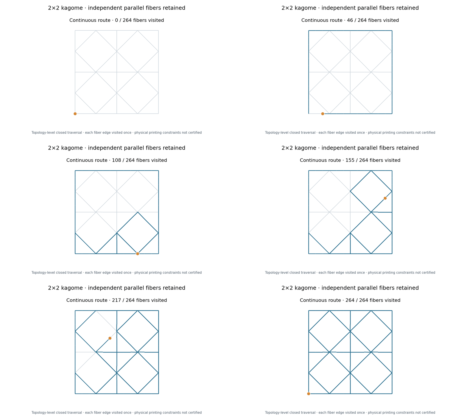
The orange point follows the library's closed Euler route through the same 2×2 kagome graph. Blue segments have already been visited; gray segments remain. Every independent fiber edge is counted once, including parallel fibers. The editable final SVG and source and parameter manifest are provided. This is a graph traversal, not a printer motion or a bond-quality test.
Export a bounded solid and route file
Install optional geometry dependencies with python -m pip install -e ".[manufacturing]", then run python -m examples.solid_export_workflow --output-dir demo_solid. The executable example generates a small closed solid and writes binary STL, millimeter 3MF, an edge-ordered route CSV, and a JSON summary. It checks the triangle count, 3MF unit, and positive closed-mesh volume after export. The desktop APP uses the same geometry and export core; printer handoff and interactive controls remain APP functions. This example verifies file format and topology, not a printer-specific process window.
Desktop application
The FiberScope 3.1 Windows x64 download is a ZIP containing the tested desktop executable and its runtime files; extract the whole folder before starting FiberScope.exe. The desktop guide covers its English-default interface and shared recruitment workflow. The ZIP is a Windows build; the Python package is installed separately from PyPI. Optional SAC/TD3/DDPG training requires an external configured Python runtime and is not bundled into the executable. English and Chinese interface screenshots document the workflow pages.
Reproduce and extend
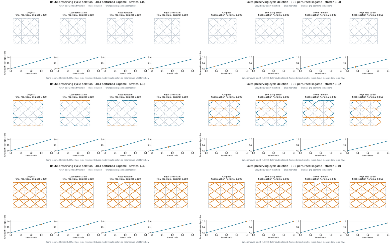
The 3×3 perturbed kagome example contains 436 nodes and 576 fibers before intervention. All four panels use the same original graph and loading; three deletion choices each remove the same 1.00% edge-length class and retain an Euler route. The low-early-strain and fixed-random choices retain approximately the original final reduced-model reaction, while the high-late-strain choice has a ratio of 0.850 in this one case. The larger network makes the local edge changes and evolving grip-spanning component visible within a representative simulation sized like the main stretch animation. Inspect the editable final-frame SVG and source/parameter manifest. Rebuild with python scripts/make_intervention_media.py --case kagome:seed23:x after completing the study checkpoint. This numerical contrast is model-specific: the same-graph independent FEM comparison does not support a general safe-deletion claim.
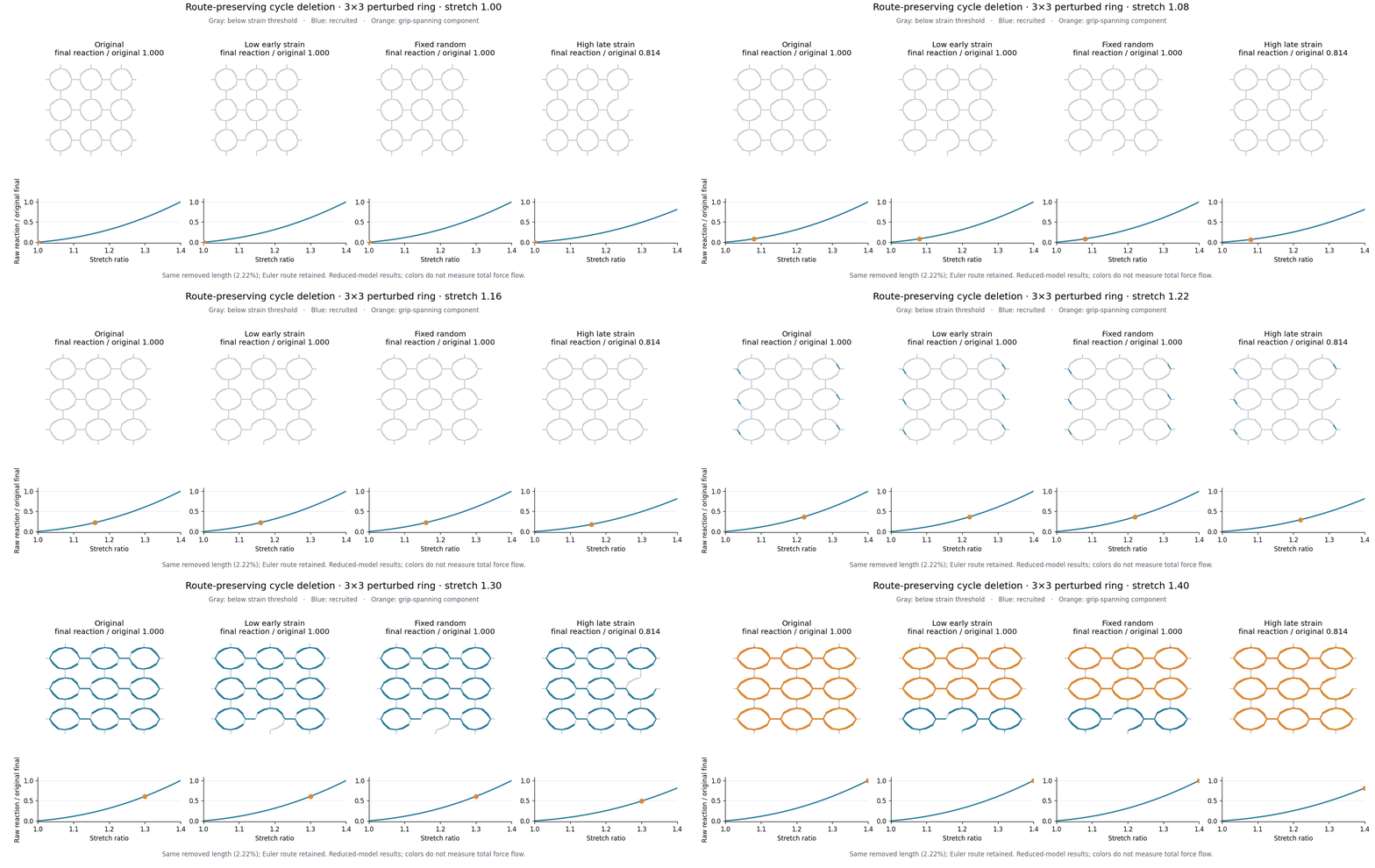
The companion 3×3 perturbed ring uses a matched 2.22% removed edge length. Each remaining graph has a constructed Euler route; the high-late-strain deletion has a smaller final raw reaction in this one numerical case, while the low-early and fixed-random choices are nearly indistinguishable. The colored edges in both animations show thresholded positive axial strain, not full force flow. Inspect the editable final-frame SVG, source and parameter manifest, and full study report. Rebuild this second animation with python scripts/make_intervention_media.py --case ring:seed11:x.
The repository contains graph-level tests, numerical golden comparisons, APP workflow tests, source-index JSON, and Methods documents. The route-preserving intervention study now compares five selection rules on 24 loading configurations, with strictly matched removed length, an explicitly reconstructed Euler route, and a separate reduced-solver run after each distinct deletion. Early low-strain selection did not consistently beat a static geometry rule or fixed random choice; this is a reproducible research example rather than a material optimization claim.
To inspect the study from a source checkout, run python benchmarks/constrained_cycle_intervention.py --output study_cycle.json --max-cases 1; rerun without --max-cases to continue the same atomically saved checkpoint. The script rejects incompatible parameters or source signatures on resume. A complete default study uses four topologies, three base-geometry seeds and two loading directions; x and y share each base structure and must not be counted as independent material specimens. The editable five-page paper work deck contains measured intervention and cross-model summaries; it is a research work file, not a final publication figure set.
The topology-held-out AI cycle study reruns all 408 eligible cycle deletions and compares an early-feature random forest with the non-trained rules on the actual post-deletion response. It is a research benchmark rather than a stable general-purpose API; python benchmarks/ai_cycle_selector.py resumes its atomically saved result and rejects stale source or reference data. Its AI and static-geometry selections have nearly identical average response in this numerical cohort, so the page does not present AI as a proven material improvement.
An independent linear beam-FEM deletion check re-simulates the same 24 configurations at a common stretch ratio of 1.08, with the same clamp node IDs in both models. On the kagome cases, early low-strain deletion retains about 1.000 of the original raw reaction in the reduced model but 0.842 in the beam model on average. This disagreement makes model assumptions visible; neither model is an experimental ground truth. Reproduce the bounded, resumable screen with python benchmarks/independent_fem_cycle_intervention.py after the cycle reference checkpoint exists.
License and attribution
The project uses the MIT license; dependency and model notices are in FiberScope/THIRD_PARTY_NOTICES.md. Existing scientific contributions are described in the published Nature Communications article. The proposed platform Methods work addresses software interoperability and a separate dynamic recruitment study; it does not reintroduce the article's original topology and inverse-design claims as new.
1 maintainer

Metadata
1 maintainer
Release files for fibernet 4.2.0
For a detailed explanation of source distributions (sdists) and built distributions (wheels), please see the package formats documentation.
Source distribution (sdist)
| File | Size | Uploaded | |
|---|---|---|---|
| fibernet-4.2.0.tar.gz | 16.6 MB | Details |
Built distribution (wheel)
| File | Interpreter | ABI | Platform | Reset |
|---|---|---|---|---|
| fibernet-4.2.0-py3-none-any.whl | Python 3 | none | any | Details |
Total release size: 17.3 MB
Release files / fibernet-4.2.0.tar.gz
| Download URL | fibernet-4.2.0.tar.gz |
|---|---|
| Size | 16.6 MB |
| Tags | Source |
|
SHA-256 checksum How to use checksums |
c924a466b463d0ad712c7655bcf7463884a944db5be9c13a365f985574ab6788
|
|
BLAKE2b-256 checksum How to use checksums |
3a4563d4dbaffd44441d983879b091aca69ad950395baed65164420fca59a514
|
| Upload date | |
|
Uploaded using Trusted Publishing? What is trusted publishing? |
No |
| Uploaded via |
twine/7.0.0 CPython/3.10.9
|
Release files / fibernet-4.2.0-py3-none-any.whl
| Download URL | fibernet-4.2.0-py3-none-any.whl |
|---|---|
| Size | 716.6 kB |
| Tags | Python 3 |
|
SHA-256 checksum How to use checksums |
7b526b8bf6a5e281a8ab07108236b8574f12cac6bfcfee70b5c581770bd4b4fd
|
|
BLAKE2b-256 checksum How to use checksums |
0fb751aab75ee752af973258e517540ae188776fd96b1166c1543199647592f8
|
| Upload date | |
|
Uploaded using Trusted Publishing? What is trusted publishing? |
No |
| Uploaded via |
twine/7.0.0 CPython/3.10.9
|

















