
FigWorks
FigWorks assembles multi-panel publication figures from Matplotlib plots, VecTeX equations, VecView 3D scenes, VecWire circuit schematics, and native SVG elements. The figure is generated from code and stays editable afterwards: panels and elements keep stable ids, the same script writes byte-identical SVG, and the result opens in Inkscape for final adjustments.
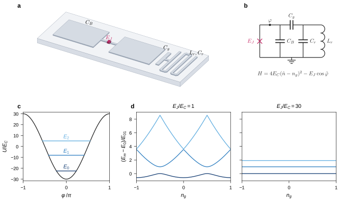
A Physical Review two-column figure from examples/transmon_figure.py: a VecView device, a VecWire circuit, and two Matplotlib panels, labelled with VecTeX.
The four sources in that figure share nothing but a method, and FigWorks composes them in a few lines:
theme = load_theme("aps")
fig = Figure(width=theme.page["double"], height="104mm", theme=theme)
panels = fig.grid(
    [["device", "device", "circuit"], ["potential", "bands", "bands"]],
    height_ratios=(1.1, 1),
    margins=("6mm", "3mm", "10mm", "12mm"),  # top, right, bottom, left
    gap=("13mm", "14mm"),  # between rows, between columns
)

labels = {name: vectex.render(source, size_pt=8) for name, source in tex.items()}

panels["device"].add(device_scene(labels), id="device-scene")  # a vecview.Scene
for name in ("EJ", "CB", "Cg", "res"):
    fig.fill_slot(f"label-{name}", labels[name])  # pinned in 3D, still 8 pt

panels["circuit"].add(circuit_diagram(labels), id="circuit", fit="none")  # at its own size

mpl_fig, ax = panels["potential"].subplots()  # its axes frame is the panel
plot_potential(ax)
panels["potential"].add(mpl_fig, id="potential-plot", fit="axes")

mpl_fig, axes = panels["bands"].subplots(1, 2, sharey=True, gridspec_kw=dict(wspace=0.12))
plot_bands(axes)
panels["bands"].add(mpl_fig, id="bands-plot", fit="axes")

for letter, panel in zip("abcd", panels.values(), strict=True):
    fig.label(letter, panel.nw)
fig.save("transmon_figure.pdf")
device_scene returns a vecview.Scene, circuit_diagram a vecwire.Circuit,
and the plot functions are plain Matplotlib, all in the example. The grid fixes
the panels in millimetres, the plots' frames land exactly on them, the circuit
is placed at the size it was drawn, so every label prints at the style's 8 pt,
and the export refuses to substitute a missing font.
SVG is the canonical output; PDF and PNG are exported through CairoSVG. FigWorks is an assembly layer between plotting code and the final graphic. It does not replace Matplotlib, TeX, Inkscape, or Illustrator.
FigWorks is alpha: the core figure model works and is tested, but the API is still settling and a minor release may change it.
Install
FigWorks is on PyPI and needs Python 3.12 or newer:
python -m pip install figworks
This pulls in Matplotlib, lxml, svg.py, CairoSVG, and VecTeX. Rendering
equations with VecTeX also needs a TeX installation with pdflatex and
dvisvgm on PATH, and MuPDF's mutool with a current Ghostscript
(mupdf-tools on Debian and Ubuntu). VecView
and VecWire are optional. VecView is on
PyPI; VecWire is installed from GitHub:
python -m pip install "vecview>=0.3"
python -m pip install "vecwire @ git+https://github.com/maiani/vecwire"
Figures are set in TeX Gyre Heros by default, a free Helvetica clone that comes
with TeX Live and as fonts-texgyre on Debian and Ubuntu. PDF and PNG export
check, through fontconfig, that every font a figure uses is installed and has
every glyph it needs, and raise FontError rather than substitute silently.
Quick start
Two plots in one Physical Review column, needing only Matplotlib:
import matplotlib.pyplot as plt
import numpy as np

from figworks import Figure
from figworks.matplotlib import theme_rc

plt.rcParams.update(theme_rc("aps"))  # Matplotlib in the figure's face and sizes

fig = Figure(width="86mm", height="42mm", theme="aps")  # one Physical Review column
panels = fig.grid([["power", "phase"]], margins=("5mm", "2mm", "10mm", "13mm"), gap="15mm")

detuning = np.linspace(-4, 4, 200)
response = 1 / (1 + 2j * detuning)
for name, curve, ylabel in (
    ("power", abs(response) ** 2, r"$|S_{21}|^2$"),
    ("phase", np.angle(response), r"$\arg S_{21}$ (rad)"),
):
    mpl_fig, ax = panels[name].subplots()  # its axes frame is exactly the panel
    (line,) = ax.plot(detuning, curve)
    line.set_gid(f"{name}-curve")  # survives into the SVG, for selectors and Inkscape
    ax.set_xlabel(r"$\Delta/\kappa$")
    ax.set_ylabel(ylabel)
    panels[name].add(mpl_fig, id=f"{name}-plot", fit="axes")

fig.label("a", panels["power"].nw)
fig.label("b", panels["phase"].nw)
fig.select("#phase-curve").set_style(stroke="#c2185b")  # edit by id after composing
fig.save("resonance.svg")
fig.save("resonance.pdf")
fig.save("resonance.png", dpi=600)
The two frames are the same size and sit level, however wide their tick labels.
Coordinates and sizes accept px, pt, mm, cm, or in; bare numbers are
px. The curve ids survive composition, so a selector reaches the phase curve
inside its placed plot, and Inkscape finds it by the same id.
For the common case of dropping SVG into existing Matplotlib axes, compose
needs no Figure at all:
import figworks
import matplotlib.pyplot as plt

fig, ax = plt.subplots()
ax.plot([0, 1], [0, 1])
svg = figworks.compose({ax: "logo.svg"}, fig=fig)
with open("figure.svg", "w", encoding="utf-8") as output:
    output.write(svg)
What it does
The root package exports Figure, Panel, Anchor, Theme, compose,
layout_svgs, display_svg, and FigureCollection. With them you can:
- create an SVG canvas with physical dimensions and a style:
"paper","presentation", the journal styles"nature","aps", and"ieee", or your ownstyle.md; - divide it into named panels with
Figure.grid, or place panels by hand; - add rectangular panels with named anchors (
panel.nw,panel.center, …); - place Matplotlib figures, VecTeX fragments, VecView scenes, VecWire circuits,
SVG files, and SVG strings through one call,
Panel.add; - add native text, panel labels, rectangles, lines, circles, ellipses, polylines, paths, and arrows;
- reserve placeholders and fill them by id later;
- lay out many SVGs into a labelled grid;
- select elements by
#id,.class, or tag name, then delete them or set attributes and inline style, which reaches the leaves a source styled itself; - save to
.svg,.pdf, and.png, byte-identically from run to run, and display figures inline in notebooks; - regenerate a whole set of figures from one command with
FigureCollection.
Panel.add reads each source's intrinsic size from its viewBox, scales it
uniformly, and centres it in the panel; fit="none" keeps the size the source
declares instead, so an 8 pt label prints at 8 pt, and align picks the point
of the panel it sits on. Placement wraps the source in a group
and keeps its ids, prefixing only those that collide with ids already in the
figure, so selectors reach inside placed content.
Sources
Everything except Matplotlib integrates through one method: FigWorks places any
object exposing to_svg_document(). VecTeX, VecView, and VecWire implement it
without importing FigWorks, and FigWorks has no adapter for any of them.
VecTeX equations
import vectex

equation = vectex.render(r"\[E = mc^2\]", id_prefix="equation")
panel.add(equation, id="equation-panel")
fig.select("#equation-root").set_attr("color", "navy")  # VecTeX glyphs use currentColor
VecView scenes
import vecview

cam = vecview.OrthographicCamera(azim_deg=35, elev_deg=24, scale=62)
scene = vecview.Scene(cam, pad=6)
slab = vecview.box_faces(center=(0, 0, -0.45), size=(11, 9, 0.9))
scene.faces(10, slab, cull=True, fill="#cfd6e0")

panel.add(scene, id="slab-scene")
Leave the scene's background unset and keep pad small: the scene is scaled
to fit its panel, so padding shrinks the drawing.
A scene can also hold content of its own. Scene.plane reserves a rectangle of
a world plane and Figure.fill_plane puts a plot in it, foreshortened with
the geometry. Scene.slot pins an empty, upright group to a world point and
Figure.fill_slot fills it with content kept at its own physical size, so an
8 pt TeX label stays 8 pt however the scene was scaled:
scene.plane(15, origin=(-4.2, -2.9, 0.01), u_edge=(0, 8.4, 0), v_edge=(5.8, 0, 0), id="plot-plane")

label = vectex.render(r"$\hat{z}$", size_pt=8)
scene.slot(45, (5.5, 4.5, 0), label.width_px, label.height_px, align="west", dx=1.6, id="label-z")

panel.add(scene, id="device")
fig.fill_plane("plot-plane", mpl_fig)
fig.fill_slot("label-z", label)
fill_plane normalizes content onto the unit square, so shape the plane to the
plot's aspect ratio. 3D scenes covers orientation,
line weights, and export caveats.
VecWire circuits
A vecwire.Circuit places like any other source, and its component ids and
data-component attributes survive placement:
right = fig.panel("schematic", x="120mm", y="8mm", w="40mm", h="56mm")
right.add(circuit, id="transmon-circuit")
fig.select("#JJ")  # a junction drawn with id="JJ"
One style document per publication
---
base: aps            # or nature, ieee, paper, presentation, another style.md
color:
  spin_up: "#d62828"
cycle: [spin_up]
---

# Style guide: what each colour means, which weight is for what ...
A style.md holds the publication's design tokens in its YAML frontmatter and
its style guide in prose. FigWorks generates Matplotlib settings from it
(theme_rc("style.md")), styles its own elements with it
(Figure(..., theme="style.md")), and builds figure sets under it
(FigureCollection(style=...)). Built-in bases follow the figure guidelines of
Nature, Physical Review, and IEEE. See Styles.
Aligned Matplotlib panels
panel = fig.panel("a", x="18mm", y="8mm", w="62mm", h="48mm")
mpl_fig, ax = panel.subplots()  # axes frame exactly the panel, at 1:1
ax.plot(x, y)
panel.add(mpl_fig, id="plot-a", fit="axes")
Plots made this way keep their nominal text size, and their axes frames sit exactly on their panels, so frames in a row line up whatever their tick labels.
Matplotlib, both directions
from figworks.matplotlib import connect, insert, mpl_to_svg

svg = mpl_to_svg(mpl_fig)  # Matplotlib -> SVG
connect(ax, "slot", 0.2, 0.2, 0.6, 0.6)  # reserve a placeholder in the axes
result = insert({"slot": panel_fig}, fig=mpl_fig)  # swap in vector SVG by id
Matplotlib exports are made deterministic: FigWorks pins the id salt and drops the export date, which otherwise change on every run.
Placeholders and grids
Create named panels without calculating their coordinates:
fig = Figure(width="180mm", height="110mm")
panels = fig.grid(
    [["device", "device"], ["spectrum", "response"]],
    width_ratios=(3, 2),
    height_ratios=(1, 2),
    margins=("8mm", "6mm", "12mm", "16mm"),  # top, right, bottom, left
    gap=("16mm", "22mm"),  # between rows, between columns
)
panels["device"].add(scene, id="device-scene")
mpl_fig, ax = panels["spectrum"].subplots()
ax.plot(x, y)
panels["spectrum"].add(mpl_fig, id="spectrum-plot", fit="axes")
fig.label("b", panels["spectrum"].nw)
Repeating a name spans a rectangle; None reserves an empty cell. Ratios
divide the space remaining after margins and gaps, which keep their physical
size when you build a figure at another width. The returned dictionary holds
ordinary Panel objects in first-occurrence order. See Grid layout
and the complete example.
fig.placeholder("main-slot", x="10mm", y="10mm", w="80mm", h="60mm", label="x")
fig.fill("main-slot", mpl_fig)  # a figure, an SVG file path, or an SVG string
from figworks import layout_svgs

grid = layout_svgs([svg_a, svg_b, svg_c], labels=["a", "b", "c"], outline=True)
grid.save("grid.svg")
Known limitations
A gradient-filled <mask> does not survive CairoSVG and vanishes from PDF and
PNG exports without a warning.
Examples
Run from the repository root:
python examples/transmon_figure.py      # requires vecview, vecwire, and TeX
python examples/minimal_svg.py
python examples/matplotlib_panel.py
python examples/two_panel_figure.py
python examples/panel_grid.py
python examples/matplotlib_bridge.py
python examples/vecview_panel.py         # requires vecview
python examples/vecview_plane_plot.py    # requires vecview; a plot in a 3D plane
python examples/vecwire_panel.py         # requires vecwire
Each example writes its figures into examples/out/.
The suite
FigWorks is the composition layer of four projects developed together, each independently useful:
| Project | Produces | Maturity |
|---|---|---|
| FigWorks | composed, exported multi-panel figures | alpha: core API still settling |
| VecTeX | editable TeX equations as SVG fragments | beta: on PyPI, API settled enough to build on |
| VecView | layered 3D schematics as SVG documents | alpha: on PyPI, API may change before 1.0 |
| VecWire | editable circuit schematics as SVG documents | pre-alpha: first version, on GitHub, not yet on PyPI |
All four emit vector SVG with stable ids and byte-identical output for identical input, so a figure can be regenerated from code, diffed in version control, and still hand-tuned in Inkscape. All four are pre-1.0 and make no backward-compatibility promise; deterministic output is the one guarantee they share.
The dependency edges are uneven by design: VecTeX is a runtime requirement, VecView and VecWire are optional, and none of the three depends on FigWorks.
Development
python -m venv .venv
source .venv/bin/activate
python -m pip install -e ".[dev]"
ruff format --check .
ruff check .
ty check
pytest
Tests for VecView and VecWire skip when those packages are not installed, and
tests that render VecTeX skip without pdflatex and dvisvgm.
Rendering tests need TeX Gyre Heros, DejaVu Sans, and fontconfig's command-line
tools (Debian/Ubuntu: fonts-texgyre fonts-dejavu-core fontconfig).
Documentation
The docs in docs/ are built with Zensical:
zensical serve    # preview at http://localhost:8000
zensical build    # static build into site/
License
MIT
1 maintainer

Metadata
1 maintainer
Release files for figworks 0.8.0
For a detailed explanation of source distributions (sdists) and built distributions (wheels), please see the package formats documentation.
Source distribution (sdist)
| File | Size | Uploaded | |
|---|---|---|---|
| figworks-0.8.0.tar.gz | 71.5 kB | Details |
Built distribution (wheel)
| File | Interpreter | ABI | Platform | Reset |
|---|---|---|---|---|
| figworks-0.8.0-py3-none-any.whl | Python 3 | none | any | Details |
Total release size: 124.2 kB
Release files / figworks-0.8.0.tar.gz
| Download URL | figworks-0.8.0.tar.gz |
|---|---|
| Size | 71.5 kB |
| Tags | Source |
|
SHA-256 checksum How to use checksums |
7c937a5d6d6583ccd3a2d49834d7c78a3ff9669d3ca6379056458a185619a8c2
|
|
BLAKE2b-256 checksum How to use checksums |
724a80227347f4a7038170d303b9367d5d804dbe8c425633c99c4ee951b8b6f6
|
| Upload date | |
|
Uploaded using Trusted Publishing? What is trusted publishing? |
Yes |
| Uploaded via |
twine/7.0.0 CPython/3.13.14
|
Provenance
Provenance describes where a file came from. On PyPI, provenance is shared via attestations, which provide a verifiable record of the build or publishing details. View details, limitations and caveats.


PyPI Publish Attestation
PyPI verified that this artifact, at this checksum, originated from the publisher listed below.
Signed by GitHub Actions, verified by PyPI on Oct 8, 2026.
Transparency logRelease files / figworks-0.8.0-py3-none-any.whl
| Download URL | figworks-0.8.0-py3-none-any.whl |
|---|---|
| Size | 52.6 kB |
| Tags | Python 3 |
|
SHA-256 checksum How to use checksums |
f685cb2bfbf6013264689ddf344d3e6e5ee5a8ba972956564452af30a8c45230
|
|
BLAKE2b-256 checksum How to use checksums |
a066ab7e186165911371a064301b97df6bd161315d0f3bd0e97f1b7a326d4394
|
| Upload date | |
|
Uploaded using Trusted Publishing? What is trusted publishing? |
Yes |
| Uploaded via |
twine/7.0.0 CPython/3.13.14
|
Provenance
Provenance describes where a file came from. On PyPI, provenance is shared via attestations, which provide a verifiable record of the build or publishing details. View details, limitations and caveats.
PyPI Publish Attestation
PyPI verified that this artifact, at this checksum, originated from the publisher listed below.
Signed by GitHub Actions, verified by PyPI on Oct 8, 2026.
Transparency log













