filter-optimizer 0.2

Optimize digital filters with differential evolution

Author:

Ralf Schlatterbeck <[e-mail]>

This project originated when I was learning digital filter design from the book “Digital Signal Processing” [1] recommended to me by a colleague.

The main idea here is the optimization of digital filters (with additional constraints on group delay variation) with Differential Evolution (DE) inspired by an early paper on the subject by Rainer Storn [2], [3].

It also includes various Jupyter notebooks where I was experimenting with what I’d learned. These include:

• IIR_Filter.ipynb: Various filter examples I could get my hands on to test my implementations of pole-zero plots, frequency response and group delay. It also includes the outcome of my attempts at optimizing filters with Differential Evolution (DE) inspired by an early paper on the subject by Rainer Storn [2] (the paper is behind a paywall, you may want to read the technical report [3] which has all information in the paper and is available online from ICSI, unfortunately as of this writing it seems the report is no longer available)

• Experiments.ipynb: Here I tried conversion of analog filters to their digital counterparts. In addition I was experimenting with a method for minimizing group delay variance.

• RIAA.ipynb: This has experiments with various digital filters for the RIAA equalization used in vinyl players. The digital filter can never fully match the analog filter (although I’m sure nobody my age can ever hope to hear the difference). This analyzes RIAA implementations from various sources.

Example call

The optimizer takes options for upper and lower bounds on the filter magnitude by frequency (in dB) as well as on the group delay (in samples). The options for the filter magnitude are -u and -l for upper and lower bound, respectively. The options for the group delay are (capital) -U and -L for upper and lower bound, respectively. These take four mandatory parameters: The minimum and maximum X-value, the minimum and maximum Y-value. In addition the number of points can be specified and another optional parameter if a raised cosine transform should be applied (this makes the points tighter at the bounds).

Experiment without pre-filter, this is from the Storn paper [3]:

mpirun --machinefile ~/.mpi-openmpi-cat  --np 8 \
python3 -m filter_optimizer.filter_optimizer \
-u 0,0.04938,0.01,0.025,9 -u 0.04938,0.2716,0.025,0.025,73 \
-u 0.2716,0.3334,0.05,0.05,151 -u 0.3334,0.395,-12,-12,43 \
-u 0.395,0.5,-40,-40,37 \
-l 0.0,0.04938,-0.01,-0.025,9 -l 0.04938,0.2716,-0.025,-0.025,43 \
-l 0.2716,0.284,-0.05,-0.05 \
-U 0.0,0.284,0.10125,0.30375,17 -L 0.0,0.284,-0.10125,-0.30375,50 \
-R2 >! by2.out

The result in by2.out can be plotted with the command:

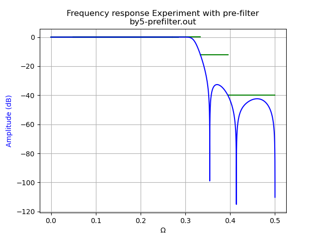
filter-show-from-log by5-prefilter.out

resulting in the magnitude graph in the following figure. Note that this program is interactive and we can zoom into the graph – which unfortunately is not possible here.

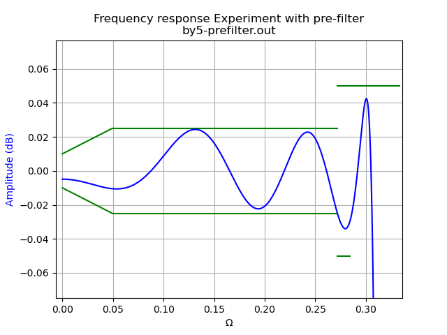
The green lines indicate the specified magnitude bounds while the blue line is the filter magnitude. The X-axis is the frequency in units of the sampling rate. The passband cannot be seen clearly so this is magnified in the following graph

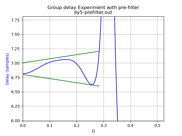
The group delay is shown in the next figure

Again the green lines show the bounds while the blue line reflects the delay in samples. Note that the delay specification to the algorithm is not in absolute samples but relative to the middle of the delay.

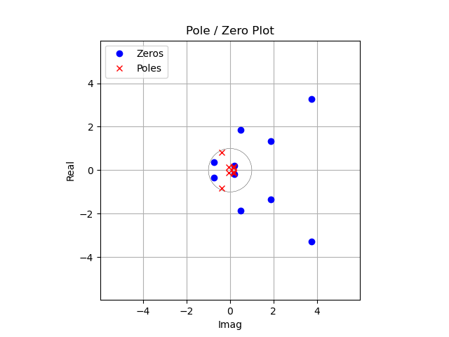
The pole zero plot for this filter can be seen in the next figure

The same experiment can be run with a pre-filter, in the paper [3] an existing filter is asumed (the magnitude response of the pre-filter is shown in the IIR-Filter jupyter notebook) and the goal is to design a second filter so that both filter together fulfill the requirements. We see that we get a completely different filter (e.g. when looking at the pole-zero plot) but it still fulfills the requirements:

mpirun --machinefile ~/.mpi-openmpi-cat  --np 8 \
python3 -m filter_optimizer.filter_optimizer --use-prefilter \
-u 0,0.04938,0.01,0.025,9 -u 0.04938,0.2716,0.025,0.025,73 \
-u 0.2716,0.3334,0.05,0.05,151 -u 0.3334,0.395,-12,-12,43 \
-u 0.395,0.5,-40,-40,37 \
-l 0.0,0.04938,-0.01,-0.025,9 -l 0.04938,0.2716,-0.025,-0.025,43 \
-l 0.2716,0.284,-0.05,-0.05 \
-U 0.0,0.284,0.10125,0.30375,17 -L 0.0,0.284,-0.10125,-0.30375,50 \
-R5 >! by5-prefilter.out

The next two are solutions to the specification of a high pass filter also with some group delay constraints also from a paper that optimizes filters with Differential Evolution [4] but using it for optimizing analog filters. I’ve added an upper limit of 2.5 dB for the transition band ripple. I leave it to the reader to plot the results:

mpirun --machinefile ~/.mpi-openmpi-cat  --np 8 filter-optimizer \
-P 7 -Z 7 -u 0,1,-70,-70,100 -u 1,1.5,2.5,2.5,100 \
-l1.5,3.14159265,-0.075,-0.075,31,1 \
-u 1.5,3.14159265,0.075,0.075,31,1 -L 1.5,3.14159265,-1.25,-1.25,100 \
-U 1.5,3.14159265,1.25,1.25,100 --dont-scale-by-pi -R6 >! 06vond.out

mpirun --machinefile ~/.mpi-openmpi-cat  --np 8 filter-optimizer \
-P 7 -Z 7 -u 0,1,-70,-70,100,0,0.9542 -u 1,1.5,2.5,2.5,100 \
-l1.5,3.14159265,-0.075,-0.075,31,1 \
-u 1.5,3.14159265,0.075,0.075,31,1 -L 1.5,3.14159265,-1.25,-1.25,100 \
-U 1.5,3.14159265,1.25,1.25,100 --dont-scale-by-pi -R6 >! 06vond+1x.out

Finally we have another example of a high-pass filter with tighter constraints in the transition band:

mpirun --machinefile ~/.mpi-openmpi-cat  --np 8 filter-optimizer \
-P 7 -Z 7 -u 0,1,-70,-70,100 -u 1,1.5,0.075,0.075,100,0,1.174 \
-l1.5,3.14159265,-0.075,-0.075,31,1 \
-u 1.5,3.14159265,0.075,0.075,31,1 -L 1.5,3.14159265,-1.25,-1.25,100 \
-U 1.5,3.14159265,1.25,1.25,100 --dont-scale-by-pi \
-R8 >!  hi-constraint-8+1.out

When we zoom in we find that the constraints seem to be violated at certain positions, we see two peaks overflowing the upper green line and also the lower green line seems to be violated.

To see what is going on we can use the --scatter option when plotting. Instead of a line we only show the individual positions where we actually test the bounds. We see that due to the raised cosine distribution of points we actually have huge gaps in the points where we test the boundaries.

And even the seemingly high violation happens to pass between two test points. So when setting up the bounds you should check that the number of test points is high enough and verify that no violations occur.

[1]

John G. Proakis and Dimitris G. Manolakis. Digital Signal Processing: Principles, Algorithms, and Applications. Pearson Prentice Hall, Upper Saddle River, New Jersey, fourth edition, 2007.

[2] (1,2)

Rainer Storn. Differential evolution design of an IIR-filter. In IEEE International Conference on Evolutionary Computation (ICEC), pages 268–273, Nagoya, Japan, May 1996.

[3] (1,2,3,4)

Rainer Storn. Differential evolution design of an IIR-filter with requirements for magnitude and group delay. Technical Report TR-95-026, International Computer Science Institute (ICSI), June 1995. Available online from ICSI – as of this writing the links seems to be down.

[4]

Jan Vondras and Pravoslav Martinek. Multi-criterion filter design via differential evolution method for function minimization. In IEEE International Conference on Circuits and Systems for Communications (ICCSC), pages 106–109, St. Petersburg, Russia, 2002.