Transparent and Efficient Financial Analysis

Project description


While browsing a variety of websites, I kept finding that the same financial metric can greatly vary per source and so do the financial statements reported while little information is given how the metric was calculated.
For example, Microsoft's Price-to-Earnings (PE) ratio on the 6th of May, 2023 is reported to be 28.93 (Stockopedia), 32.05 (Morningstar), 32.66 (Macrotrends), 33.09 (Finance Charts), 33.66 (Y Charts), 33.67 (Wall Street Journal), 33.80 (Yahoo Finance) and 34.4 (Companies Market Cap). All of these calculations are correct, however the method applied varies leading to different results. Therefore, collecting data from multiple sources can lead to wrong interpretation of the results given that one source could be applying a different calculation method than another. And that is, if it is even freely available. Often the calculation is hidden behind a paid subscription.
This is why I designed the FinanceToolkit, this is an open-source toolkit in which all relevant financial ratios (100+), indicators and performance measurements are written down in the most simplistic way allowing for complete transparency of the calculation method. This allows you to not have to rely on metrics from other providers and, given a financial statement, allow for efficient manual calculations. This leads to one uniform method of calculation being applied that is available and understood by everyone.
The Finance Toolkit is complimented very well with the Finance Database 🌎, a database that features 300.000+ symbols containing Equities, ETFs, Funds, Indices, Currencies, Cryptocurrencies and Money Markets. By utilising both, it is possible to do a fully-fledged competitive analysis with the tickers found from the FinanceDatabase inputted into the FinanceToolkit.

Table of Contents
Installation
Before installation, consider starring the project on GitHub which helps others find the project as well.
To install the FinanceToolkit it simply requires the following:
pip install financetoolkit
Then within Python use:
from financetoolkit import Toolkit
To be able to get started, you need to obtain an API Key from FinancialModelingPrep. This is used to gain access to 30+ years of financial statement both annually and quarterly. Note that the Free plan is limited to 250 requests each day, 5 years of data and only features companies listed on US exchanges.
Through the link you are able to subscribe for the free plan and also premium plans at a 15% discount. This is an affiliate link and thus supports the project at the same time. I have chosen FinancialModelingPrep as a source as I find it to be the most transparent, reliable and at an affordable price. I have yet to find a platform offering such low prices for the amount of data offered. When you notice that the data is inaccurate or have any other issue related to the data, note that I simply provide the means to access this data and I am not responsible for the accuracy of the data itself. For this, use their contact form or provide the data yourself.
Basic Usage
This section explains in detail how the Finance Toolkit can utilitised effectively. Also see the Jupyter Notebooks in which you can run the examples also demonstrated here.
Within this package the following things are included:
- Company profiles (
get_profile), including country, sector, ISIN and general characteristics (from FinancialModelingPrep) - Company quotes (
get_quote), including 52 week highs and lows, volume metrics and current shares outstanding (from FinancialModelingPrep) - Company ratings (
get_rating), based on key indicators like PE and DE ratios (from FinancialModelingPrep) - Historical market data (
get_historical_data), which can be retrieved on a daily, weekly, monthly and yearly basis. This includes OHLC, dividends, returns, cumulative returns and volatility calculations for each corresponding period. (from Yahoo Finance) - Treasury Rates (
get_treasury_data) for several months and several years over the last 3 months which allows yield curves to be constructed (from FinancialModelingPrep) - Analyst Estimates (
get_analyst_estimates) that show the expected EPS and Revenue from the past and future from a range of analysts (from FinancialModelingPrep) - Earnings Calendar (
get_earnings_calendar) which shows the exact dates earnings are released in the past and in the future including expectations (from FinancialModelingPrep) - Revenue Geographic Segmentation (
get_revenue_geographic_segmentation) which shows the revenue per company from each country and Revenue Product Segmentation (get_revenue_product_segmenttion) which shows the revenue per company from each product (from FinancialModelingPrep) - Balance Sheet Statements (
get_balance_sheet_statement), Income Statements (get_income_statement), Cash Flow Statements (get_cash_flow_statement) and Statistics Statement (get_statistics_statement), obtainable from FinancialModelingPrep or the source of your choosing through custom input. These functions are accompanied with a normalization function so that for any source, the same ratio analysis can be performed. Please see this Jupyter Notebook that explains how to use a custom source. - Efficiency ratios (
ratios.collect_efficiency_ratios), liquidity ratios (ratios.collect_liquidity_ratios), profitability ratios (ratios._collect_profitability_ratios), solvency ratios (ratios.collect_solvency_ratios) and valuation ratios (ratios.collect_valuation_ratios) functionality that automatically calculates the most important ratios based on the inputted balance sheet, income and cash flow statements. Any of the underlying ratios can also be called individually such asratios.get_return_on_equity. Next to that, it is also possible to input your own custom ratios (ratios.collect_custom_ratios). See also this Notebook or this section for more information. - Models like DUPONT analysis (
models.get_extended_dupont_analysis) or Enterprise Breakdown (models.get_enterprise_value_breakdown) that can be used to perform in-depth financial analysis through a single function. These functions combine much of the functionality throughout the Toolkit to provide advanced calculations. - Technical indicators like Relative Strength Index (
technicals.get_relative_strength_index), Exponential Moving Average (models.get_exponential_moving_average) and Bollinger Bands (technicals.get_bollinger_bands) that can be used to perform in-depth momentum and trend analysis. These functions allow for the calculation of technical indicators based on the historical market data.
The dependencies of the package are on purpose very slim so that it will work well with any combination of packages and not result in conflicts.
Using the Finance Toolkit
A basic example of how to initialise the Finance Toolkit is shown below, also see this notebook for a detailed Getting Started guide as well as this notebook that includes the Finance Database 🌎 and a proper financial analysis.
from financetoolkit import Toolkit

companies = Toolkit(['AAPL', 'MSFT'], api_key="FMP_KEY", start_date='2017-12-31')

# a Historical example
historical_data = companies.get_historical_data()

# a Financial Statement example
balance_sheet_statement = companies.get_balance_sheet_statement()

# a Ratios example
profitability_ratios = companies.ratios.collect_profitability_ratios()

# a Models example
extended_dupont_analysis = companies.models.get_extended_dupont_analysis()

# a Technical example
bollinger_bands = companies.technicals.get_bollinger_bands()
For each object, it returns a multi-index in which both Apple and Microsoft are presented. For this example, I've selected just Apple to keep things organized but in essence it can be any list of tickers (no limit). The filtering is done through using .loc['AAPL'] and .xs('AAPL', level=1, axis=1) based on whether it's fundamental data or historical data respectively.
Historical Data
Obtain historical data on a daily, weekly, monthly or yearly basis. This includes OHLC, volumes, dividends, returns, cumulative returns and volatility calculations for each corresponding period.
| Date | Open | High | Low | Close | Adj Close | Volume | Dividends | Return | Volatility | Excess Return | Excess Volatility | Cumulative Return |
|---|---|---|---|---|---|---|---|---|---|---|---|---|
| 2018-01-02 | 42.54 | 43.075 | 42.315 | 43.065 | 40.7765 | 1.02224e+08 | 0 | 0 | 0.0203524 | -0.00674528 | 0.0231223 | 1 |
| 2018-01-03 | 43.1325 | 43.6375 | 42.99 | 43.0575 | 40.7694 | 1.18072e+08 | 0 | -0.000173997 | 0.0203524 | -0.024644 | 0.0231223 | 0.999826 |
| 2018-01-04 | 43.135 | 43.3675 | 43.02 | 43.2575 | 40.9588 | 8.97384e+07 | 0 | 0.00464441 | 0.0203524 | -0.0198856 | 0.0231223 | 1.00447 |
| 2018-01-05 | 43.36 | 43.8425 | 43.2625 | 43.75 | 41.4251 | 9.464e+07 | 0 | 0.0113856 | 0.0203524 | -0.0133744 | 0.0231223 | 1.01591 |
| 2018-01-08 | 43.5875 | 43.9025 | 43.4825 | 43.5875 | 41.2713 | 8.22712e+07 | 0 | -0.00371412 | 0.0203524 | -0.0285141 | 0.0231223 | 1.01213 |
Financial Statements
Obtain a Balance Sheet Statement on an annual or quarterly basis. This can also be an income statement (companies.get_income_statement()) or cash flow statement (companies.get_cash_flow_statement()).
| 2018 | 2019 | 2020 | 2021 | 2022 | |
|---|---|---|---|---|---|
| Cash and Cash Equivalents | 2.5913e+10 | 4.8844e+10 | 3.8016e+10 | 3.494e+10 | 2.3646e+10 |
| Short Term Investments | 4.0388e+10 | 5.1713e+10 | 5.2927e+10 | 2.7699e+10 | 2.4658e+10 |
| Cash and Short Term Investments | 6.6301e+10 | 1.00557e+11 | 9.0943e+10 | 6.2639e+10 | 4.8304e+10 |
| Accounts Receivable | 4.8995e+10 | 4.5804e+10 | 3.7445e+10 | 5.1506e+10 | 6.0932e+10 |
| Inventory | 3.956e+09 | 4.106e+09 | 4.061e+09 | 6.58e+09 | 4.946e+09 |
| Other Current Assets | 1.2087e+10 | 1.2352e+10 | 1.1264e+10 | 1.4111e+10 | 2.1223e+10 |
| Total Current Assets | 1.31339e+11 | 1.62819e+11 | 1.43713e+11 | 1.34836e+11 | 1.35405e+11 |
| Property, Plant and Equipment | 4.1304e+10 | 3.7378e+10 | 3.6766e+10 | 3.944e+10 | 4.2117e+10 |
| Goodwill | 0 | 0 | 0 | 0 | 0 |
| Intangible Assets | 0 | 0 | 0 | 0 | 0 |
| Long Term Investments | 1.70799e+11 | 1.05341e+11 | 1.00887e+11 | 1.27877e+11 | 1.20805e+11 |
| Tax Assets | 0 | 0 | 0 | 0 | 0 |
| Other Fixed Assets | 2.2283e+10 | 3.2978e+10 | 4.2522e+10 | 4.8849e+10 | 5.4428e+10 |
| Fixed Assets | 2.34386e+11 | 1.75697e+11 | 1.80175e+11 | 2.16166e+11 | 2.1735e+11 |
| Other Assets | 0 | 0 | 0 | 0 | 0 |
| Total Assets | 3.65725e+11 | 3.38516e+11 | 3.23888e+11 | 3.51002e+11 | 3.52755e+11 |
| Accounts Payable | 5.5888e+10 | 4.6236e+10 | 4.2296e+10 | 5.4763e+10 | 6.4115e+10 |
| Short Term Debt | 2.0748e+10 | 1.624e+10 | 1.3769e+10 | 1.5613e+10 | 2.111e+10 |
| Tax Payables | 0 | 0 | 0 | 0 | 0 |
| Deferred Revenue | 7.543e+09 | 5.522e+09 | 6.643e+09 | 7.612e+09 | 7.912e+09 |
| Other Current Liabilities | 3.2687e+10 | 3.772e+10 | 4.2684e+10 | 4.7493e+10 | 6.0845e+10 |
| Total Current Liabilities | 1.16866e+11 | 1.05718e+11 | 1.05392e+11 | 1.25481e+11 | 1.53982e+11 |
| Long Term Debt | 9.3735e+10 | 9.1807e+10 | 9.8667e+10 | 1.09106e+11 | 9.8959e+10 |
| Deferred Revenue Non Current | 2.797e+09 | 0 | 0 | 0 | 0 |
| Deferred Tax Liabilities | 4.26e+08 | 0 | 0 | 0 | 0 |
| Other Non Current Liabilities | 4.4754e+10 | 5.0503e+10 | 5.449e+10 | 5.3325e+10 | 4.9142e+10 |
| Total Non Current Liabilities | 1.41712e+11 | 1.4231e+11 | 1.53157e+11 | 1.62431e+11 | 1.48101e+11 |
| Other Liabilities | 0 | 0 | 0 | 0 | 0 |
| Capital Lease Obligations | 0 | 0 | 0 | 0 | 0 |
| Total Liabilities | 2.58578e+11 | 2.48028e+11 | 2.58549e+11 | 2.87912e+11 | 3.02083e+11 |
| Preferred Stock | 0 | 0 | 0 | 0 | 0 |
| Common Stock | 4.0201e+10 | 4.5174e+10 | 5.0779e+10 | 5.7365e+10 | 6.4849e+10 |
| Retained Earnings | 7.04e+10 | 4.5898e+10 | 1.4966e+10 | 5.562e+09 | -3.068e+09 |
| Accumulated Other Comprehensive Income | -3.454e+09 | -5.84e+08 | -4.06e+08 | 1.63e+08 | -1.1109e+10 |
| Other Total Shareholder Equity | 0 | 0 | 0 | 0 | 0 |
| Total Shareholder Equity | 1.07147e+11 | 9.0488e+10 | 6.5339e+10 | 6.309e+10 | 5.0672e+10 |
| Total Equity | 1.07147e+11 | 9.0488e+10 | 6.5339e+10 | 6.309e+10 | 5.0672e+10 |
| Total Liabilities and Shareholder Equity | 3.65725e+11 | 3.38516e+11 | 3.23888e+11 | 3.51002e+11 | 3.52755e+11 |
| Minority Interest | 0 | 0 | 0 | 0 | 0 |
| Total Liabilities and Equity | 3.65725e+11 | 3.38516e+11 | 3.23888e+11 | 3.51002e+11 | 3.52755e+11 |
| Total Investments | 2.11187e+11 | 1.57054e+11 | 1.53814e+11 | 1.55576e+11 | 1.45463e+11 |
| Total Debt | 1.14483e+11 | 1.08047e+11 | 1.12436e+11 | 1.24719e+11 | 1.20069e+11 |
| Net Debt | 8.857e+10 | 5.9203e+10 | 7.442e+10 | 8.9779e+10 | 9.6423e+10 |
Financial Ratios
Get Profitability Ratios based on the inputted balance sheet, income and cash flow statements. This can be any of the 50+ ratios within the ratios module. The get_ functions show a single ratio whereas the collect_ functions show an aggregation of multiple ratios.
| 2018 | 2019 | 2020 | 2021 | 2022 | |
|---|---|---|---|---|---|
| Gross Margin | 0.3834 | 0.3782 | 0.3823 | 0.4178 | 0.4331 |
| Operating Margin | 0.2669 | 0.2457 | 0.2415 | 0.2978 | 0.3029 |
| Net Profit Margin | 0.2241 | 0.2124 | 0.2091 | 0.2588 | 0.2531 |
| Interest Coverage Ratio | 25.2472 | 21.3862 | 26.921 | 45.4567 | 44.538 |
| Income Before Tax Profit Margin | 0.2745 | 0.2527 | 0.2444 | 0.2985 | 0.302 |
| Effective Tax Rate | 0.1834 | 0.1594 | 0.1443 | 0.133 | 0.162 |
| Return on Assets (ROA) | 0.1628 | 0.1632 | 0.1773 | 0.2697 | 0.2829 |
| Return on Equity (ROE) | nan | 0.5592 | 0.7369 | 1.4744 | 1.7546 |
| Return on Invested Capital (ROIC) | 0.2699 | 0.2937 | 0.3441 | 0.5039 | 0.5627 |
| Return on Capital Employed (ROCE) | 0.306 | 0.2977 | 0.3202 | 0.496 | 0.6139 |
| Return on Tangible Assets | 0.5556 | 0.6106 | 0.8787 | 1.5007 | 1.9696 |
| Income Quality Ratio | 1.3007 | 1.2558 | 1.4052 | 1.0988 | 1.2239 |
| Net Income per EBT | 0.8166 | 0.8406 | 0.8557 | 0.867 | 0.838 |
| Free Cash Flow to Operating Cash Flow Ratio | 0.8281 | 0.8488 | 0.9094 | 0.8935 | 0.9123 |
| EBT to EBIT Ratio | 0.9574 | 0.9484 | 0.9589 | 0.9764 | 0.976 |
| EBIT to Revenue | 0.2867 | 0.2664 | 0.2549 | 0.3058 | 0.3095 |
Financial Models
Get an Extended DuPont Analysis based on the inputted balance sheet, income and cash flow statements. This can also be for example an Enterprise Value Breakdown (companies.models.get_enterprise_value_breakdown()).
| 2017 | 2018 | 2019 | 2020 | 2021 | 2022 | |
|---|---|---|---|---|---|---|
| Interest Burden Ratio | 0.9572 | 0.9725 | 0.9725 | 0.988 | 0.9976 | 1.0028 |
| Tax Burden Ratio | 0.7882 | 0.8397 | 0.8643 | 0.8661 | 0.869 | 0.8356 |
| Operating Profit Margin | 0.2796 | 0.2745 | 0.2527 | 0.2444 | 0.2985 | 0.302 |
| Asset Turnover | nan | 0.7168 | 0.7389 | 0.8288 | 1.0841 | 1.1206 |
| Equity Multiplier | nan | 3.0724 | 3.5633 | 4.2509 | 5.255 | 6.1862 |
| Return on Equity | nan | 0.4936 | 0.5592 | 0.7369 | 1.4744 | 1.7546 |
Technical Indicators
Get Bollinger Bands based on the historical market data. This can be any of the 30+ technical indicators within the technicals module. The get_ functions show a single indicator whereas the collect_ functions show an aggregation of multiple indicators.
| Date | Lower Band | Middle Band | Upper Band |
|---|---|---|---|
| 2023-08-22 | 170.336 | 178.524 | 186.712 |
| 2023-08-23 | 173.376 | 177.824 | 182.272 |
| 2023-08-24 | 173.56 | 177.441 | 181.322 |
| 2023-08-25 | 173.56 | 177.441 | 181.323 |
| 2023-08-28 | 173.486 | 177.486 | 181.487 |
Defining Custom Ratios
The Finance Toolkit has an abundance of financial ratios, however it could be that you are looking for a specific ratio that is currently not provided. First and foremost, I encourage you to create a Pull Request to add these ratios in but there is also an option to add custom ratios as follows. Find a Notebook example here.
Define how each custom ratio needs to be calculated. This can be any of the following structures:
- Simple operations such as:
'Quick Assets': 'Cash and Short Term Investments + Accounts Receivable' - Working with multiple operations:
'Cash Op Expenses':'Cost of Goods Sold + Selling, General and Administrative Expenses - Depreciation and Amortization', - Using curly brackets:
'WC / Net Income as %': '(Working Capital / Net Income) * 100', - Defining a criteria:
'Large Revenues': 'Revenue > 1000000000', - Using actual numbers:
'Daily Cash Op Expenses': 'Cash Op Expenses / 365', - Combining earlier defined formulas:
'Defensive Interval':'Quick Assets / Daily Cash Op Expenses'
Not that it is important you follow the NAME - FORMULA format and that you adhere to the normalization files naming. This can be viewed relatively easy by initializing the Toolkit and running for example get_balance_sheet_statement.
custom_ratios = {
    'WC / Net Income as %': '(Working Capital / Net Income) * 100',
    'Large Revenues': 'Revenue > 1000000000',
    'Quick Assets': 'Cash and Short Term Investments + Accounts Receivable',
    'Cash Op Expenses':'Cost of Goods Sold + Selling, General and Administrative Expenses '
    '- Depreciation and Amortization',
    'Daily Cash Op Expenses': 'Cash Op Expenses / 365',
    'Defensive Interval':'Quick Assets / Daily Cash Op Expenses'
}
Initializing the Finance Toolkit. Make sure to set the parameter custom_ratios with the above dictionary. Note that quarterly=True doesn't work without a Premium plan.
from financetoolkit import Toolkit

# Initialize the Finance Toolkit
companies = Toolkit(
    ["AAPL", "MSFT", "GOOGL", "AMZN"], api_key="FMP_KEY", start_date="2022-08-10",
    custom_ratios=custom_ratios, quarterly=True
)

# Obtain the custom ratios
companies.ratios.collect_custom_ratios()
By then running ratios.collect_custom_ratios it automatically calculates the given ratios. Note the ratios Daily Cash Op Expenses and Defensive Interval which rely on an earlier defined ratio (Cash Op Expenses). This is an example of how you can create a custom ratio based on another custom ratio.
Below you can find the custom ratios from AMZN (Amazon) which has been selected with .loc['AMZN]. The Notebook as found here shows the full output.
| 2022Q4 | 2023Q1 | 2023Q2 | 2023Q3 | |
|---|---|---|---|---|
| Cash Op Expenses | 2.1856e+10 | 1.9972e+10 | 2.1322e+10 | nan |
| Daily Cash Op Expenses | 5.98795e+07 | 5.47178e+07 | 5.84164e+07 | nan |
| Defensive Interval | 2260.22 | 2592.34 | 2738.1 | nan |
| Large Revenues | 1 | 1 | 1 | 0 |
| Quick Assets | 1.35341e+11 | 1.41847e+11 | 1.5995e+11 | nan |
| WC / Net Income as % | 463.349 | 427.335 | 398.924 | nan |
In case you forgot a ratio or would like to insert new ratios, you can directly pass the custom_ratios dictionary to the function.
new_custom_ratios = {
    'WC / Net Income': 'Working Capital / Net Income',
    'Low Revenues': 'Revenue < 1000000000',
    'Quick Assets': 'Cash and Short Term Investments + Accounts Receivable',
    'Cash Op Expenses':'Cost of Goods Sold + Selling, General and Administrative Expenses '
    '- Depreciation and Amortization',
    'Monthly Cash Op Expenses': 'Cash Op Expenses / 30',
    'Defensive Interval':'Quick Assets / Monthly Cash Op Expenses'
}

# Return the new ratios by passing the dictionary into the function
companies.ratios.collect_custom_ratios(custom_ratios_dict=new_custom_ratios)
Which returns the following for GOOGL (Google):
| 2022Q3 | 2022Q4 | 2023Q1 | 2023Q2 | 2023Q3 | |
|---|---|---|---|---|---|
| Cash Op Expenses | 3.6925e+10 | 4.2495e+10 | 3.6722e+10 | 3.7896e+10 | nan |
| Defensive Interval | 123.847 | 108.733 | 123.472 | 124.395 | nan |
| Low Revenues | 0 | 0 | 0 | 0 | 0 |
| Monthly Cash Op Expenses | 1.23083e+09 | 1.4165e+09 | 1.22407e+09 | 1.2632e+09 | nan |
| Quick Assets | 1.52435e+11 | 1.5402e+11 | 1.51138e+11 | 1.57136e+11 | nan |
| WC / Net Income | 7.19842 | 7.00932 | 6.1877 | 4.95857 | nan |
Calling Functions Directly
It also possible to call any ratio or model directly as shown below. This allows access to 100+ ratios and indicators with custom data. Also see this notebook.
import pandas as pd
import numpy as np

from financetoolkit.models import dupont

years = [2018, 2019, 2020, 2021, 2022]

dupont.get_dupont_analysis(
    net_income=pd.Series(
        [59531000000, 55256000000, 57411000000, 94680000000, 99803000000], index=years
    ),
    total_revenue=pd.Series(
        [265595000000, 260174000000, 274515000000, 365817000000, 394328000000],
        index=years,
    ),
    total_assets_begin=pd.Series(
        [np.nan, 365725000000, 338516000000, 323888000000, 351002000000],
        index=years,
    ),
    total_assets_end=pd.Series(
        [365725000000, 338516000000, 323888000000, 351002000000, 352755000000],
        index=years,
    ),
    total_equity_begin=pd.Series(
        [np.nan, 107147000000, 90488000000, 65339000000, 63090000000], index=years
    ),
    total_equity_end=pd.Series(
        [107147000000, 90488000000, 65339000000, 63090000000, 50672000000], index=years
    ),
)
This returns the following table which closely resembles a proper Dupont analysis for Apple at their given reporting dates in October:
| 2018 | 2019 | 2020 | 2021 | 2022 | |
|---|---|---|---|---|---|
| Net Profit Margin | 0.224142 | 0.212381 | 0.209136 | 0.258818 | 0.253096 |
| Asset Turnover | nan | 0.738878 | 0.828845 | 1.08408 | 1.12064 |
| Equity Multiplier | nan | 3.56334 | 4.25089 | 5.25497 | 6.18622 |
| Return on Equity | nan | 0.559172 | 0.736856 | 1.47443 | 1.75459 |
Working with other Datasets
The Finance Toolkit has the ability to leverage custom datasets from any data provider as well. This makes it possible to work with your preferred data and not be limited to the data source the Finance Toolkit currently provides. A detailed example can be found here but to get started see the code below.
from financetoolkit import Toolkit

# Initialize the Finance Toolkit
companies = Toolkit(['AAPL', 'MSFT'])

# Copy the normalization files
companies.get_normalization_files()
This copies over three files, balance.csv, income.csv, cash.csv and statistics.csv (not required) which will contain a structure like the following:
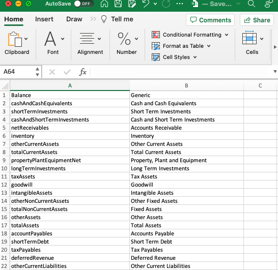
By replacing the first column with the names from your dataset (e.g. replace cashAndCashEquivalents with Cash if this is how it is called in your dataset), it will automatically normalize the dataset when you initialize the Finance Toolkit. Note that the DataFrame needs to be a multi-index in case you use multiple tickers structured as Ticker x Financial Statement Item x Periods.
As an example:
If you have individual DataFrames for each company, you can do the following which will return the DataFrame structure that is required:
from financetoolkit.base import helpers

balance_sheets = helpers.combine_dataframes(
    {
        "TSLA": tsla_balance,
        "GOOGL": googl_balance,
    },
)
income_statements = helpers.combine_dataframes(
    {
        "TSLA": tsla_income,
        "GOOGL": googl_income,
    },
)
cash_flow_statements = helpers.combine_dataframes(
    {
        "TSLA": tsla_cash,
        "GOOGL": googl_cash
    },
)
Once all of this is set-up you can feed this information to the Toolkit and use the Toolkit as normally.
# Initialize the Toolkit
companies = Toolkit(
tickers=["TSLA", "GOOGL"],
balance=balance_sheets,
income=income_statements,
cash=cash_flow_statements,
format_location="examples/external_datasets",
reverse_dates=True, # Important when the dates are descending
)
# Return all Ratios
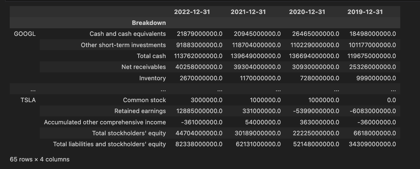
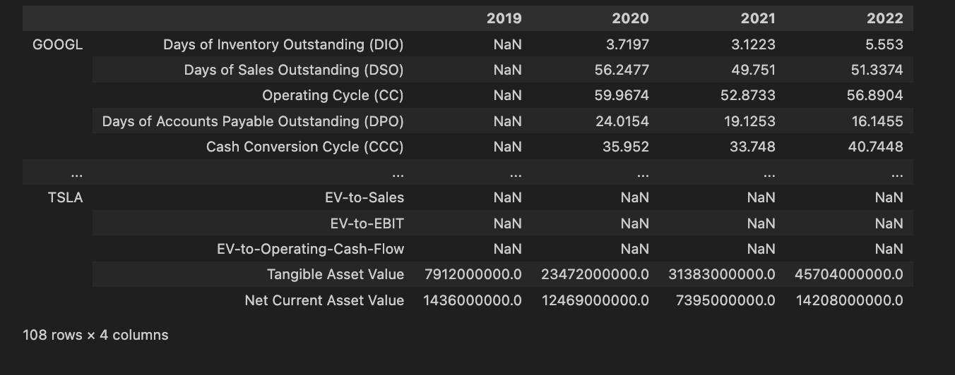
companies.ratios.collect_all_ratios()
This will return all financial ratios that can be collected based on the provided data and the format. See this notebook to understand how to work with actual datasets.
Available Ratios and Indicators
The Finance Toolkit has the ability to calculate 100+ ratios and indicators. The following list shows all of the available ratios and indicators. Note that the Finance Toolkit is not limited to these ratios and indicators as it is possible to add custom ratios as well. See this section for more information.
Each ratio and indicator has a corresponding function that can be called directly for example ratios.get_return_on_equity or technicals.get_relative_strength_index.
Financial Ratios
The Ratios Module contains over 50+ ratios that can be used to analyse companies. These ratios are divided into 5 categories which are efficiency, liquidity, profitability, solvency and valuation. Each ratio is calculated using the data from the Toolkit module. Find the documentation here which includes an explanation about the ratio, the parameters and an example.
Efficiency Ratios
- Asset Turnover Ratio
- Inventory Turnover Ratio
- Days of Inventory Outstanding
- Days of Sales Outstanding
- Operating Cycle
- Accounts Payables Turnover Ratio
- Days of Accounts Payable Outstanding
- Cash Conversion Cycle
- Receivables Turnover
- SGA to Revenue Ratio
- Fixed Asset Turnover
- Operating Ratio
Liquidity Ratios
- Current Ratio
- Quick Ratio
- Cash Ratio
- Working Capital
- Operating Cash Flow Ratio
- Operating Cash Flow Sales Ratio
- Short Term Coverage Ratio
Profitability Ratios
- Gross Margin
- Operating Margin
- Net Profit Margin
- Interest Burden Ratio
- Income Before Tax Profit Margin
- Effective Tax Rate
- Return on Assets (RoA)
- Return on Equity (RoE)
- Return on Invested Capital (RoIC)
- Income Quality Ratio
- Return on Tangible Assets (RoTA)
- Return on Capital Employed (RoCE)
- Net Income per EBT
- Free Cash Flow Operating Cash Flow Ratio
- Tax Burden Ratio
- EBT to EBIT
- EBIT to Revenue
Solvency Ratios
- Debt to Assets Ratio
- Debt to Equity Ratio
- Interest Coverage Ratio
- Equity Multiplier
- Debt Service Coverage Ratio
- Free Cash Flow Yield
- Net Debt to EBITDA Ratio
- Cash Flow Coverage Ratio
- CAPEX Coverage Ratio
- CAPEX Dividend Coverage Ratio
Valuation Ratios
- Earnings per Share (EPS)
- Revenue per Share (RPS)
- Price Earnings Ratio (PE)
- Price to Earnings Growth Ratio (PEG)
- Book Value per Share
- Price to Book Ratio (PB)
- Interest Debt per Share
- CAPEX per Share
- Dividend Yield
- Weighted Dividend Yield
- Price to Cash Flow Ratio (P/CF)
- Price to Free Cash Flow Ratio (P/FCF)
- Market Capitalization
- Enterprise Value
- EV to Sales Ratio
- EV to EBITDA Ratio
- EV to Operating Cashflow Ratio
- EV to EBIT
- Earnings Yield
- Payout Ratio
- Tangible Asset Value
- Net Current Asset Value
Financial Models
The Models module is meant to execute well-known models such as DUPONT and the Discounted Cash Flow (DCF) model. These models are also directly related to the data retrieved from the Toolkit module. Find the documentation here which includes an explanation about the model, the parameters and an example.
- DuPont Analysis
- Extended DuPont Analysis
- Enterprise Value Breakdown
Risk Metrics
The Risk module is meant to calculate important risk metrics such as Value at Risk (VaR), Conditional Value at Risk (cVaR), Maximum Drawdown, Correlations, Beta, GARCH, EWMA and more. This class is currently in active development and therefore not yet available.
- Value at Risk (VaR)
- Conditional Value at Risk (cVaR)
- Maximum Drawdown (MDD)
- ...
Technical Indicators
The Technicals Module contains 30+ Technical Indicators that can be used to analyse companies. These ratios are divided into 4 categories which are breadth, momentum, overlap and volatility. Each indicator is calculated using the data from the Toolkit module. Find the documentation here which includes an explanation about the indicator, the parameters and an example.
Breadth Indicators
- McClellan Oscillator
- Advancers/Decliners Ratio
- On-Balance Volume (OBV)
- Accumulation/Distribution Line (ADL)
- Chaikin Oscillator
Momentum Indicators
- Money Flow Index
- Williams %R
- Aroon Indicator
- Commodity Channel Index
- Relative Vigor Index
- Force Index
- Ultimate Oscillator
- Percentage Price Oscillator
- Detrended Price Oscillator
- Average Directional Index (ADX)
- Chande Momentum Oscillator (CMO)
- Ichimoku Cloud
- Stochastic Oscillator
- Moving Average Convergence Divergence (MACD)
- Relative Strength Index (RSI)
- Balance of Power (BOP)
Overlap Indicators
- Simple Moving Average (SMA)
- Exponential Moving Average (EMA)
- Double Exponential Moving Average (DEMA)
- Triple Exponential Moving Average (TRIX)
- Triangular Moving Average (TMA)
Volatility Indicators
- True Range (TR)
- Average True Range (ATR)
- Keltners Channels
- Bollinger Bands
Contributing
First off all, thank you for taking the time to contribute (or at least read the Contributing Guidelines)! 🚀
The goal of the Finance Toolkit is to make any type of financial calculation as transparent and efficient as possible. I want to make these type of calculations as accessible to anyone as possible and seeing how many websites exists that do the same thing (but instead you have to pay) gave me plenty of reasons to work on this.
The following is a set of guidelines for contributing to the Finance Toolkit.
Structure
The Finance Toolkit follows the Model, View, Controller model except it cuts out the View part being more focussed on calculations than on visusally depicting the data given that there are plenty of providers that offer this solution already. The MC model (as found in financetoolkit/base) is therefore constructed as follows:
- _controller modules (such as toolkit_controller and ratios_controller) orchestrate the data flow. Through the controller, the user can set parameters (such as tickers, start and end date) that define the data that needs to be obtained. E.g. in the controller classes you will be able to find the function
get_income_statementwhich collects income statements via a _model that takes in the parameters set by the user. - _model modules (such as fundamentals_model and historical_model) are the modules that actually obtain the data. E.g in the fundamentals_model exists a function called
get_financial_statementswhich would be executed byget_income_statementfrom the controller class to obtain the financial statement, in this case the income statement, for the selected parameters. These functions will also work separately, they do not need the controller to work but the controller needs them to work.
Next to that, each individual ratio, technical indicator, risk metric etc. is categorized and kept in its own directory. E.g. all functions of ratios can be found inside financetoolkit/ratios in which if I wanted to see the Price-to-Book ratio function, I'd visit the valuation.py (given that Price-to-Book ratio is categorized as a Valuation Ratio) and then scroll to the function which would be the following:
def get_price_to_book_ratio(
    price_per_share: pd.Series, book_value_per_share: pd.Series
) -> pd.Series:
    """
    Calculate the price to book ratio, a valuation ratio that compares a company's market
    price to its book value per share.

    Args:
        price_per_share (float or pd.Series): Price per share of the company.
        book_value_per_share (float or pd.Series): Book value per share of the company.

    Returns:
        float | pd.Series: The price to book ratio value.
    """
    return price_per_share / book_value_per_share
This applies to any metric and this is also how the MC model retrieves the correct input. The get_price_to_book_ratio function is called by the ratios_controller which is called by the toolkit_controller. This is the flow of the data.
The separation is done so that it becomes possible to call all functions separately making the Finance Toolkit incredibly flexible for any kind of data input.
Adding New Functionality
If you are looking to add new functionality do the following:
- Start by looking at the available modules and whether your functionality would fit inside one of the modules.
- If the answer is yes, add it to this module.
- If the answer is no, create a new module and add it there.
- Figure out whether your functionality would fit with an existing controller. E.g. did you add a new ratio? Consider adding it to the
ratios_controller.- If the answer is yes, add it to this controller.
- If the answer is no, create a new controller and add it there. Make sure to also connect the controller to the
toolkit_controllerso that it can be called from there.
- Add in the relevant docstrings (be as extensive as possible, following already created examples) and update the README if relevant.
- Add in the relevant tests (see
testsdirectory for examples). - Create a Pull Request with your new additions. See the next section how to do so.
Working with Git & Pull Requests
Any new contribution preferably goes via a Pull Request. In essence, all you really need is Git and basic understanding of how a Pull Request works. Find some resources that explain this well here:
On every Pull Request, a couple of linters will run (see here as well as unit tests for each function in the package. The linters check the code and whether it matches specific coding formatting. The tests check whether running the function returns the expected output. If any of these fail, the Pull Request can not be merged.
Following the Workflow
After setting up Git, you can fork and pull the project in.
- Fork the Project (more info)
- Using GitHub Desktop: Getting started with GitHub Desktop will guide you through setting up Desktop. Once Desktop is set up, you can use it to fork the repo!
- Using the command line: Fork the repo so that you can make your changes without affecting the original project until you're ready to merge them.
- Pull the Repository Locally (more info)
- Create your own branch (
git checkout -b feature/contribution) - Add your changes (
git add .) - Install pre-commit, this checks the code for any errors before committing (
pre-commit install) - Commit your Changes (
git commit -m 'Improve the Toolkit') - Check whether the tests still pass (
pytest tests) and if not, correct then.- When no formulas have changed or new tests have been added, you can use
pytest tests --record-mode=rewrite(please do provide reasoning in this case). - If formulas or calculations have changed, adjusts the tests inside the
testsdirectory.
- When no formulas have changed or new tests have been added, you can use
- Push to your Branch (
git push origin feature/contribution) - Open a Pull Request
Note: feel free to reach out if you run into any issues: jer.bouma@gmail.com or LinkedIn or open a GitHub Issue.
Contact
If you have any questions about the FinanceToolkit or would like to share with me what you have been working on, feel free to reach out to me via:
- Website: https://jeroenbouma.com/
- LinkedIn: https://www.linkedin.com/in/boumajeroen/
- Email: jer.bouma@gmail.com
- Discord: add me on Discord
JerBouma
If you'd like to support my efforts, either help me out by contributing to the package or Sponsor Me.

Release history Release notifications | RSS feed


Download files
Download the file for your platform. If you're not sure which to choose, learn more about installing packages.
Source Distribution
Built Distribution
Filter files by name, interpreter, ABI, and platform.
If you're not sure about the file name format, learn more about wheel file names.
Copy a direct link to the current filters
File details
Details for the file financetoolkit-1.3.2.tar.gz.
File metadata
- Download URL: financetoolkit-1.3.2.tar.gz
- Upload date:
- Size: 104.9 kB
- Tags: Source
- Uploaded using Trusted Publishing? No
- Uploaded via: twine/4.0.2 CPython/3.10.9
File hashes
| Algorithm | Hash digest | |
|---|---|---|
| SHA256 |
331b987d17bf4a65d54492b99752aa1a93838ff9ca2d7475b46b3f7ade65f040
|
|
| MD5 |
9cb1332006d7c51092c75d9803080d87
|
|
| BLAKE2b-256 |
5c78dcba51aa7d74c9da66ab39f83d293448618ea94443034381d503c00d021d
|
File details
Details for the file financetoolkit-1.3.2-py3-none-any.whl.
File metadata
- Download URL: financetoolkit-1.3.2-py3-none-any.whl
- Upload date:
- Size: 105.5 kB
- Tags: Python 3
- Uploaded using Trusted Publishing? No
- Uploaded via: twine/4.0.2 CPython/3.10.9
File hashes
| Algorithm | Hash digest | |
|---|---|---|
| SHA256 |
802a13e943ebb1f77b2e84582c9245a872e331e93425d9ed58f3b8eff0feef2c
|
|
| MD5 |
06f6707839d9d15e299001354db4e7b2
|
|
| BLAKE2b-256 |
b12c51f32a81fc8e2a3f1598a56b4b277c037826254a32fa44ddea64f1a7a80b
|


