
Optimization Engine
A multi-asset portfolio optimization engine with a clean API, a Streamlit
UI, a CLI, and an MCP server. Built on top of cvxpy, scipy, pandas
and scikit-learn, with plotting, Excel and regression support behind
optional extras.
The engine is opinionated about one thing: an allocation is not a result until you can see what it rests on. Every solve returns the weights and the evidence — which solver answered, whether the constraints were actually respected, how well-conditioned the covariance estimate was, how concentrated the book is in risk rather than capital, how much of the backtest survives out of sample, and how much of that survives the number of configurations you tried before settling on this one.
New in 0.5.0 — the engine answers to agents as well as to people. There is an MCP server exposing five tools,
--jsononoptimize,backtest,checkanddescribe, and anAGENTS.mdwritten as an API map for coding agents. No optimizer or estimator changed behaviour; one pre-flight bug did —checkwas validating a different mandate from the oneoptimizewent on to solve. Details in the release notes and the changelog.
pip install finport-optengine
from optimization_engine import (
    EngineConfig,
    OptimizerSpec,
    portfolio_diagnostics,
    prices_to_returns,
    run_engine,
    sample_dataset,
)

returns = prices_to_returns(sample_dataset())   # swap in your own price panel
run = run_engine(returns, EngineConfig(optimizer=OptimizerSpec(name="risk_parity")))

print(run.result.weights.round(3).to_string())

# The weights are half the answer. The other half is what they rest on:
diag = portfolio_diagnostics(run.result.weights, run.cov_matrix)
print(f"\nsolver             {run.result.extras['solver']}")
print(f"condition number   {run.covariance_diagnostics.condition_number:,.0f}")
print(f"effective assets   {diag.effective_n:.1f} by capital, "
      f"{diag.effective_n_risk:.1f} by risk")
US_Equity        0.025
Intl_Equity      0.023
EM_Equity        0.019
Real_Estate      0.019
Commodities      0.015
Infra            0.022
Gold             0.024
US_Treasuries    0.058
TIPS             0.070
IG_Credit        0.053
HY_Credit        0.036
EM_Debt          0.041
Cash             0.595

solver             CLARABEL
condition number   2,114
effective assets   2.7 by capital, 13.0 by risk
That last line is the whole argument in one number. The book holds 59.5% cash, so by capital it is barely three positions wide — but risk parity equalises risk, so all thirteen assets contribute. A weights table alone shows the first number and hides the second.
The import name is optimization_engine and the console script is optengine,
whichever way you install it. The core is numpy, pandas, scipy, cvxpy and
scikit-learn; plotting, Excel and regression live behind
extras.
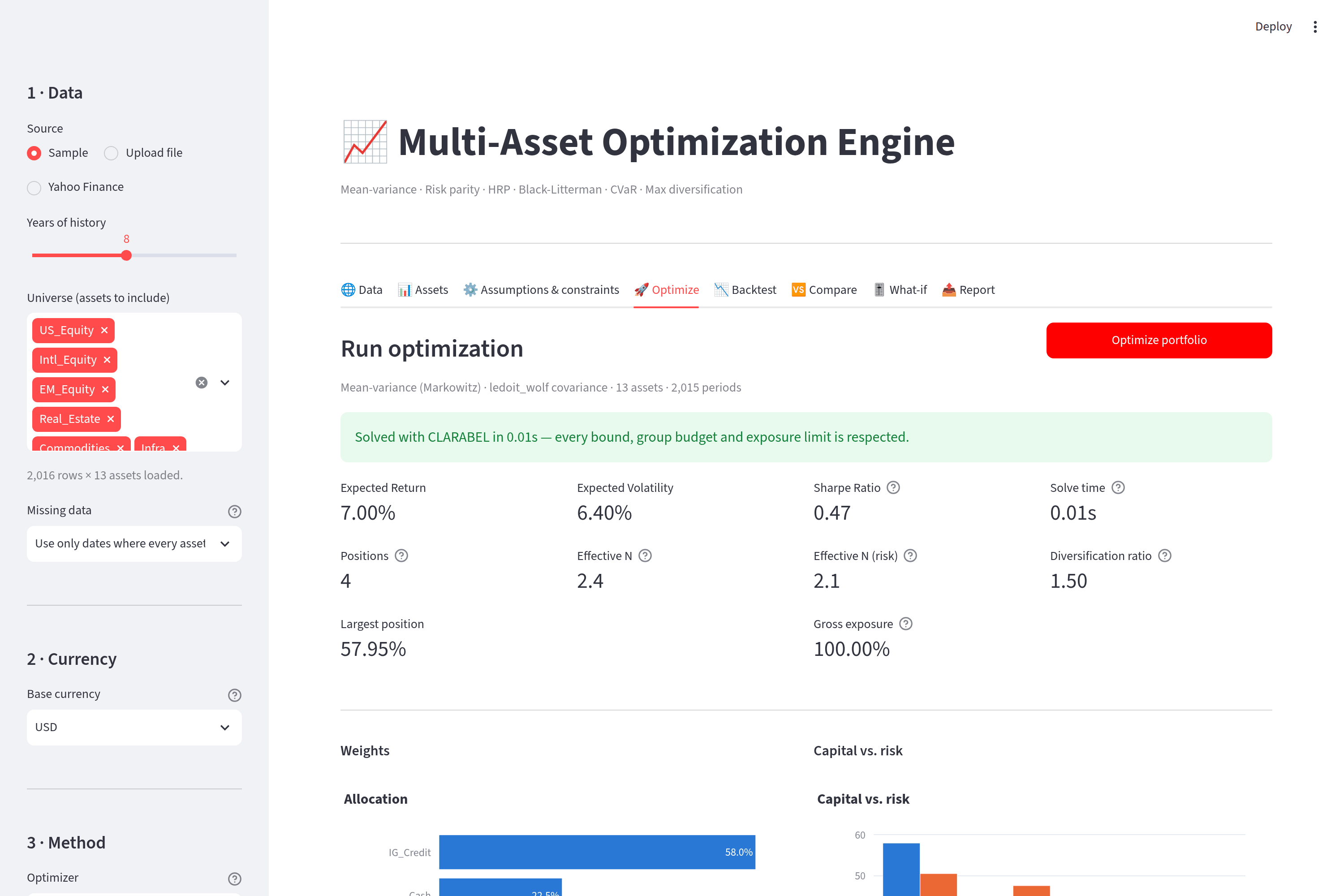
The five questions it answers
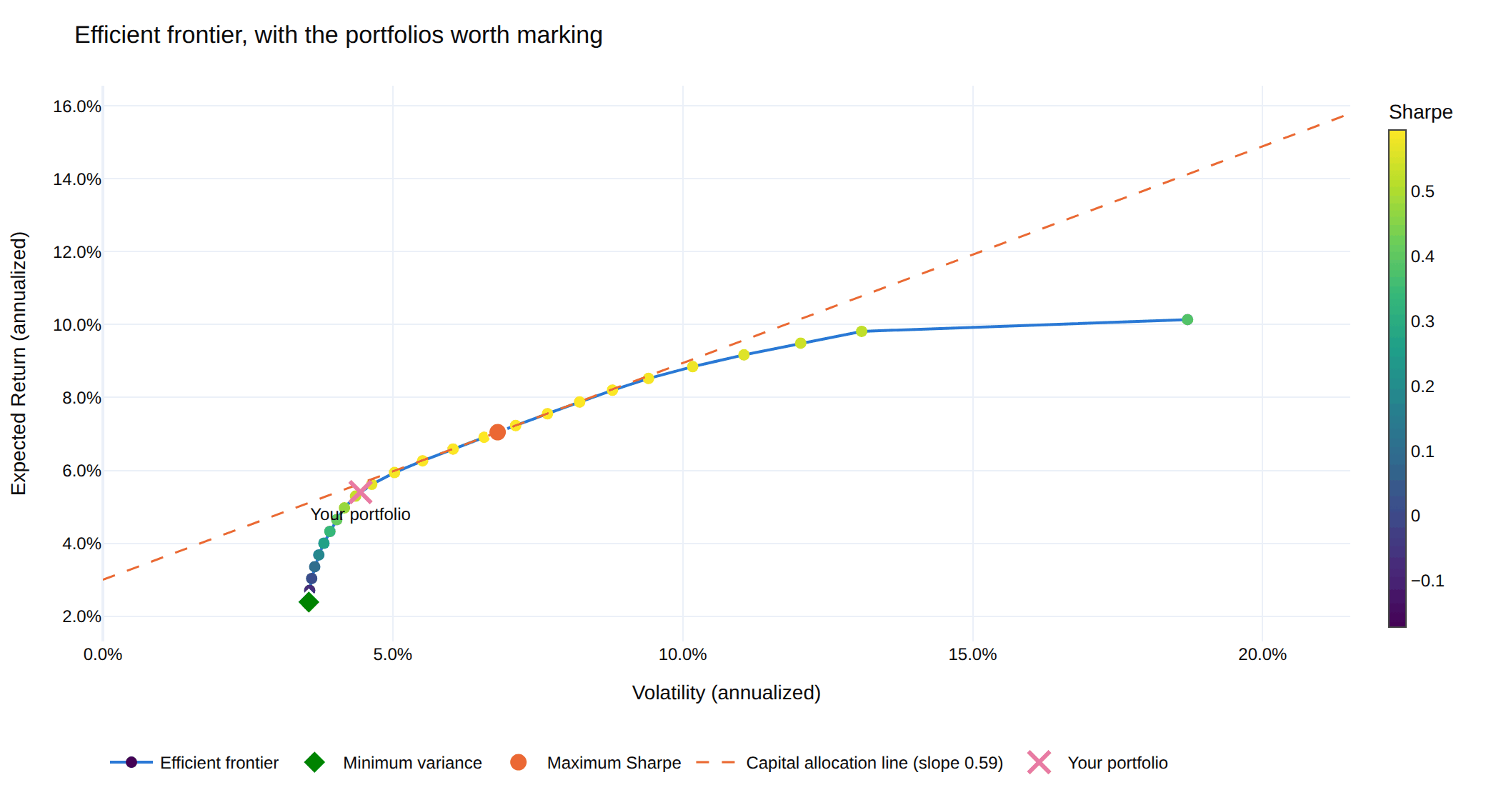
1. Where does this portfolio sit, and what else was available?
The frontier is drawn with the portfolios worth marking on it — the minimum-variance anchor where the efficient branch starts, the tangency portfolio, the capital allocation line through it, and where your own allocation actually landed. The sweep range comes from what the constraints can reach, so a binding position cap shortens the curve instead of silently failing half of it.
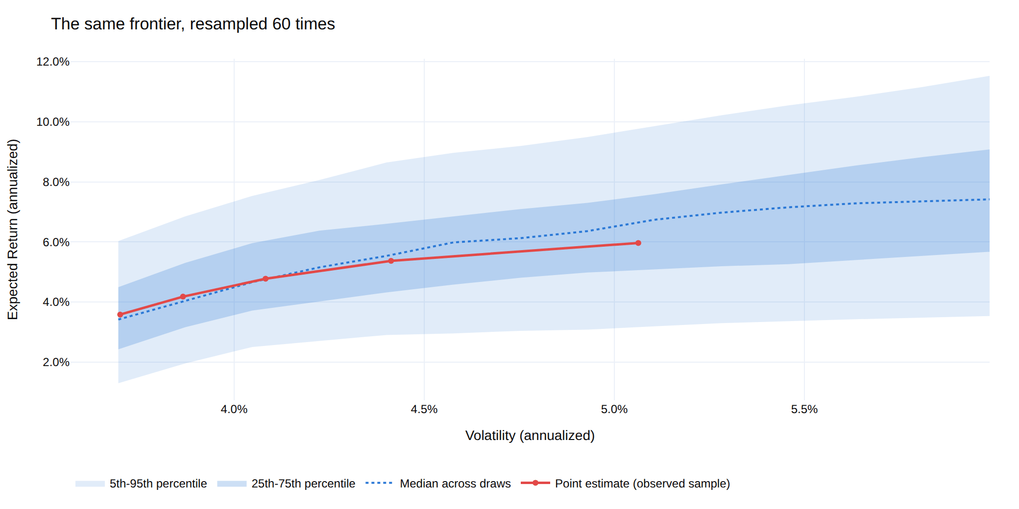
2. How much of that curve is real?
The frontier is a point estimate of a curve. Resample the return history and re-trace it, and the curve moves a great deal: on the sample panel the expected return at a typical risk level spans a 6.3-percentage-point band. Differences narrower than that band are not distinguishable from estimation noise, which is a useful thing to know before defending a 20bp allocation difference in a meeting.
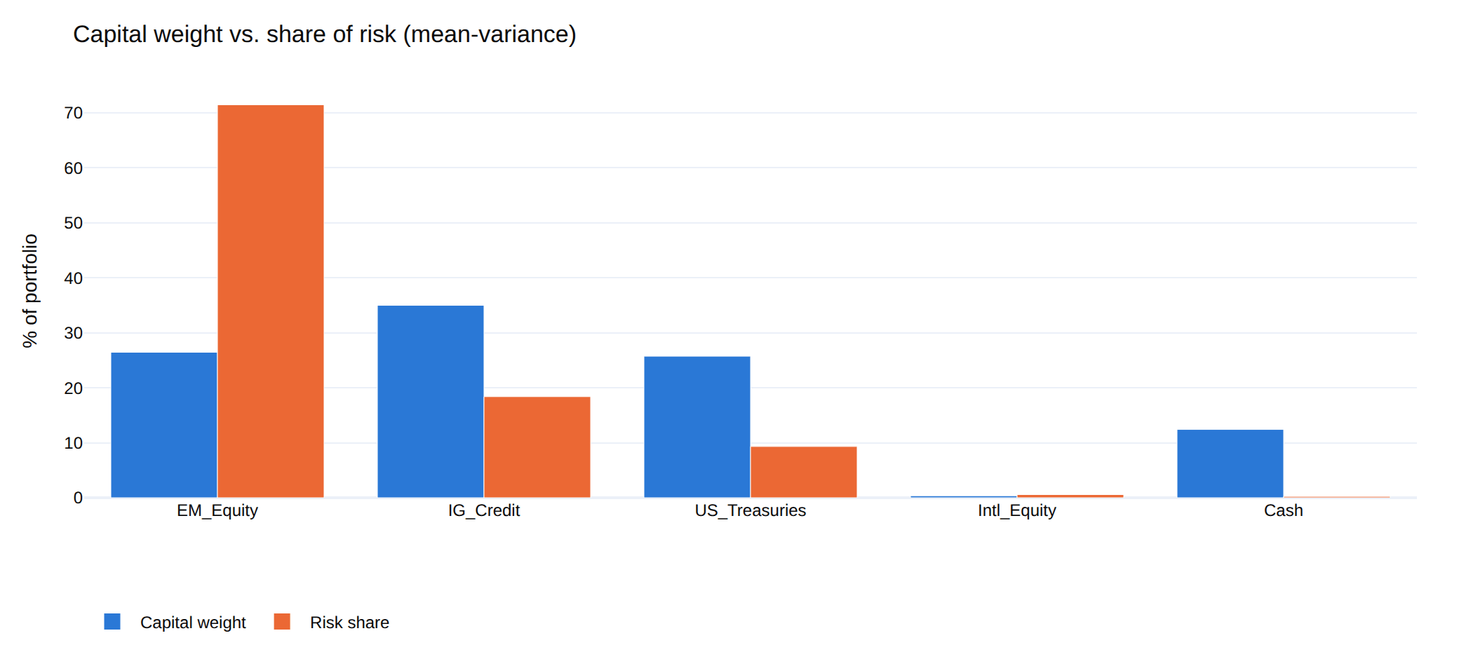
3. Where is the risk, as opposed to the money?
Capital weight and risk share are different quantities, and optimizers are happy to let them diverge. Here a 26% position in EM equity carries 71% of the portfolio's risk — the gap between the two bars is the entire argument for risk budgeting, and it is invisible in a weights table.
4. Would any of this have worked?
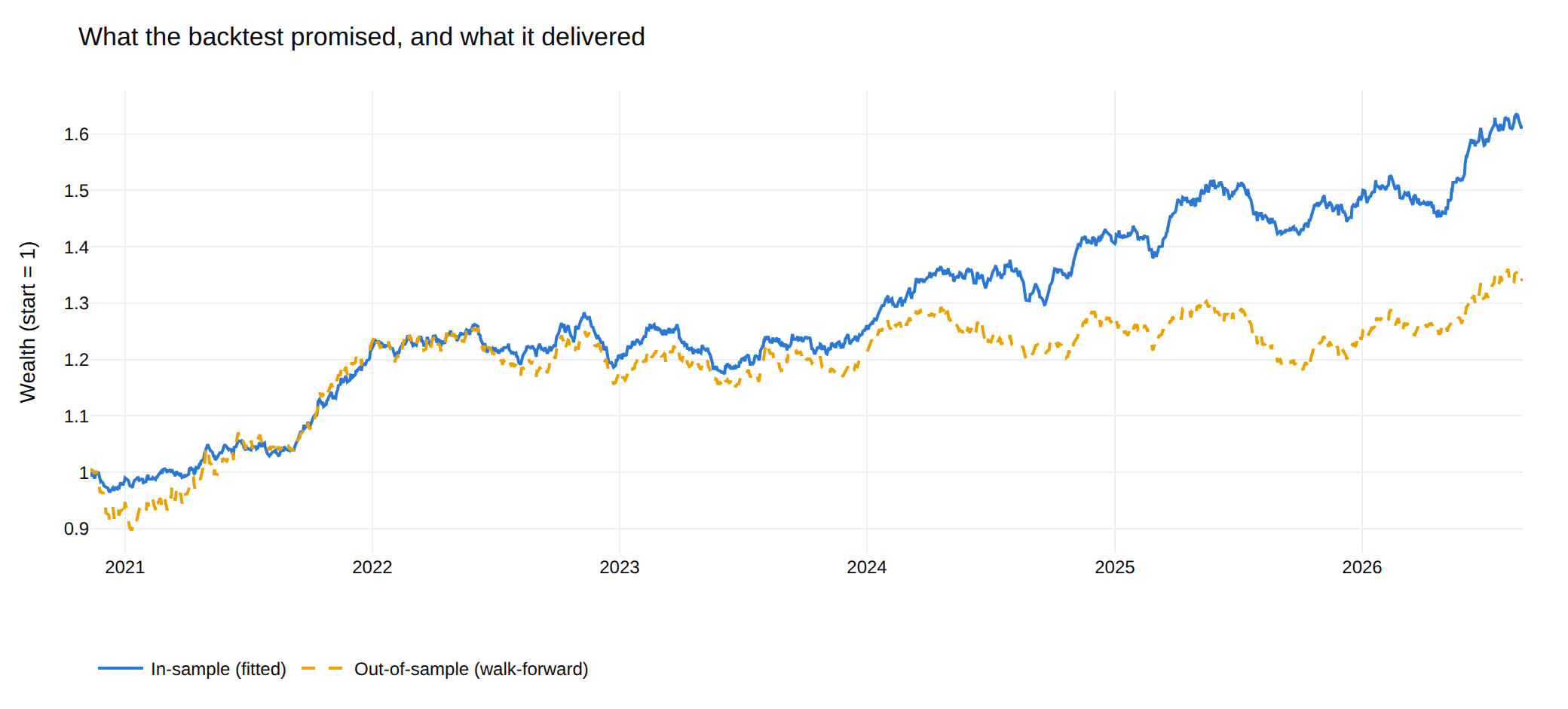
The optimizer estimated its inputs from the same returns a naive backtest replays, so a fitted track record is a description of the past, not a forecast. The walk-forward re-estimates and re-solves on a rolling window and holds each solution over returns the optimizer never saw. Same rebalancing cadence and the same 15bps of trading cost on both lines, so the gap is overfitting rather than a cost artefact: Sharpe 0.74 fitted against 0.23 walk-forward.
5. Is any of that real, or did you try forty things and report the best?
A library with ten methods, six covariance estimators and a grid of constraints makes it easy to run forty configurations and present the winner. The maximum of forty noisy estimates is a biased estimate of the best true value, and nothing about that bias shows up in the number itself.
Take 50 strategies drawn from the same zero-mean distribution — no skill anywhere. The best posts an annualized Sharpe of 1.24, and the probabilistic Sharpe ratio calls it significant at 99.3%. Deflate it for the fact that it was the best of 50 and it drops to 45.9%: a coin flip, which is what it is.
optengine optimize --trials 40 makes that declaration part of the run, and
probability_of_backtest_overfitting() asks the complementary question — across
every balanced split of the sample, how often does the in-sample winner land
below the out-of-sample median?
There is a prior question too, which monte_carlo_optimization_selection()
answers: given a universe like this one and a sample this long, which method
can be trusted to find the right answer at all? On the sample panel a direct
mean-variance solve misplaces its weights by 14.8% RMSE between simulated
histories drawn from the same distribution. Nested Clustered Optimization
misplaces them by 0.01%.
Every figure in this README is produced by python scripts/render_docs_images.py
from the built-in sample dataset, using the same plotting code the app calls —
so what the README shows is what the library draws.
What's inside
Optimization techniques
| Method | Class | When to use |
|---|---|---|
| Mean-variance (target return / vol / utility) | MeanVarianceOptimizer |
Classic Markowitz with full constraints |
| Active mean-variance (vs a benchmark) | ActiveMeanVarianceOptimizer |
The mandate is relative: excess return against an active-risk budget |
| Global minimum variance | MinVarianceOptimizer |
You don't trust any expected-return estimate |
| Maximum Sharpe ratio | MaxSharpeOptimizer |
Tangency portfolio, sized separately against cash |
| Risk parity / risk budgeting (ERC) | RiskParityOptimizer |
Spread risk evenly, not capital |
| Hierarchical Risk Parity (HRP) | HRPOptimizer |
Many assets, ill-conditioned covariance, small T/N |
| Hierarchical Equal Risk Contribution (HERC) | HERCOptimizer |
HRP's robustness, but splitting at the tree's own branches — and optionally on drawdown or tail risk |
| Nested Clustered Optimization (NCO) | NCOOptimizer |
Mean-variance keeps producing corner solutions on a correlated universe |
| Black-Litterman | BlackLittermanOptimizer |
A few specific views on top of equilibrium |
| Mean-CVaR (Rockafellar-Uryasev) | CVaROptimizer |
Skewed or fat-tailed returns; variance is the wrong measure |
| Mean-CDaR (Chekhlov-Uryasev) | CDaROptimizer |
The mandate is written in drawdown terms — a stop-loss, a high-water mark |
| Maximum diversification | MaxDiversificationOptimizer |
Correlation benefit as the objective |
| Inverse volatility | InverseVolatilityOptimizer |
Cheap risk-parity approximation |
| Equal weight (1/N) | EqualWeightOptimizer |
The baseline everything else has to beat |
optengine describe <name> prints what a method needs, what it supports, and
what it assumes — the same text the UI shows next to the method picker.
Data sources
One request goes in, one validated panel comes out, and the provider is a
string in between. Every adapter translates its vendor's schema into the same
column vocabulary, so switching providers changes a config field and nothing
else — a scenario, a benchmark reference and a constraint written against
SP500 keep working when the bytes start arriving from somewhere new.
| Provider | Key | Serves | Notes |
|---|---|---|---|
sample |
— | OHLCV | Deterministic synthetic panel. No network. The default. |
yahoo |
— | OHLCV + raw close | Total-return prices for equities, ETFs, indices, FX and crypto. One request covers the whole universe. |
stooq |
— | OHLCV | Keyless CSV history. The most dependable free source for world index levels. |
fred |
— | close only | St. Louis Fed index levels. Never carries volume, and says so. |
fmp |
free | OHLCV + VWAP | Adjusted closes for global equities, ETFs and indices. |
tiingo |
free | OHLCV | Carefully maintained adjusted end-of-day prices. Token travels in a header, never a URL. |
file |
— | anything in the file | CSV, Excel or Parquet, wide or long. |
optengine providers                       # what each can serve, and whether its key is set
optengine ingest --provider stooq \
  --identifiers "SP500, DAX, NIKKEI225" \
  --ingest-period 10y --output prices.csv
Keys follow one convention — OPTENGINE_API_KEY_<PROVIDER>, read from the
environment or a .env file — and are never logged, never raised in an
exception, and never rendered. optengine providers reports whether a key is
present, masked.
Every run returns a per-identifier log alongside the data: what loaded, from which symbol, over what span, and why anything is missing. Eleven of twelve assets arriving is not a success, and finding that out should not require counting columns.
Constraints
- Per-asset weight bounds.
- Layered allocation limits — any number of levels, all binding at once: asset class (equity ≤ 60%, fixed income ≤ 30%, commodities ≤ 10%), sub-asset class inside each of those (developed ≤ 40%, emerging ≤ 20%), and a currency split cutting across all of them (foreign FX ≤ 30%). A level's limits are read either as a share of the whole book or as a share of the parent bucket — "30% emerging" can mean 30% of the portfolio or 30% of the equity sleeve, and the second one moves with whatever the optimizer allocates to equity. Both are linear in the weights, so the problems stay convex; see Layered constraints.
- Long-only or long-short with a gross-exposure cap.
- Target return, target volatility, or risk-aversion utility.
- Turnover budget against a previous allocation.
- Tracking-error budget and active-share cap against a chosen benchmark.
Every constraint is honoured by every method, but not always the same way.
Convex solves impose them directly; the allocate-then-constrain methods (1/N,
inverse volatility, HRP) project onto the closest feasible allocation and
report how far the mandate moved their answer — because a 1/N book that had
to shift 15% of its weight is no longer really 1/N. Where a constraint truly
cannot bind (a turnover budget on the homogeneous max-Sharpe,
max-diversification and risk-parity solves), the method warns rather than
ignoring it silently. The benchmark-relative limits do carry into those
homogeneous solves: under w = y/κ an active-share cap becomes
‖y − κb‖₁ ≤ 2·AS·κ and a tracking-error budget the second-order cone
‖Σ^½(y − κb)‖₂ ≤ TE·κ, so the tangency and maximum-diversification
portfolios honour an active-risk mandate instead of reporting a breach
afterwards. After every solve the weights are checked against every
constraint and any breach is reported.
Covariance estimators
sample, ledoit_wolf, oas, ewma (RiskMetrics), semi,
shrink (an alias for ledoit_wolf), and denoised.
Every estimate is symmetrized and PSD-repaired, and comes with diagnostics: observations per asset, condition number, smallest eigenvalue, and effective sample size — with a warning when the estimate is too thin or too ill-conditioned to optimize against.
Shrinkage pulls the whole matrix toward a target, attenuating signal and noise alike. Denoising (López de Prado, 2020) is a sharper instrument: fit the Marchenko-Pastur law to the eigenvalue spectrum, replace the eigenvalues below the noise edge λ₊ with their average, and leave the factor eigenvectors untouched. Detoning additionally strips the market eigenvector, which is what the clustering methods want to see — with the market component in place every pair of equities looks alike and the hierarchy degenerates.
Both compose with any estimator (covariance_matrix(..., denoise=True, detone=1)), and both report what they found rather than what they hoped for:
Marchenko-Pastur fit on 2015 observations of 13 assets (T/N = 155.0) put the
noise edge at λ₊ = 1.167. 2 of 13 eigenvalues sit above it, carrying 62.9% of
total variance. The correlation's condition number went 18.4 → 11.2; the
covariance's went 1.25e+04 → 1.23e+04 — so this covariance's conditioning is
driven by the spread of the volatilities, not by correlation noise, and no
eigenvalue filter will improve it.
That last clause is the honest half. Denoising did what it claims and this panel's problem was somewhere else.
Expected returns
historical_mean, ema, capm, and shrunk_mean (Jorion Bayes-Stein
shrinkage toward the minimum-variance portfolio's return, which keeps the
cross-sectional ranking while pulling in the extremes that drive
mean-variance to corner solutions).
Analytics
Absolute — drawdown episodes with recovery timing, Ulcer index, time under water, VaR/CVaR (historic and Cornish-Fisher), Sharpe, probabilistic Sharpe, Sortino, Calmar, Martin, Omega, gain-to-pain, win/loss ratio, tail ratio, hit rate, best and worst single period, rolling metrics, Newey-West annualized volatility, the full Euler risk decomposition in volatility units, and concentration measures (Herfindahl, effective N, effective N of risk, diversification ratio).
Relative — annualized excess return, tracking error and its downside half, information ratio, CAPM alpha with its t-statistic and R², beta and conditional (up/down) beta, up/down capture and the up/down count ratios, batting average, Treynor, M², the appraisal ratio, relative drawdown against the benchmark's wealth curve, the probability that the true excess return is positive, and active share.
performance_report() assembles both halves into one object — headline
figures, calendar-period returns, rolling absolute and rolling relative
frames, drawdown episodes — computed on one aligned sample, which is the
point of having it. Assembling the two halves separately is how a report ends
up quoting a Sharpe ratio from ten years of history next to an information
ratio from the benchmark's shorter five, with nothing in the output saying so.
It exports as an Excel workbook or as a tidy long-form block, series, metric, value table that survives a CSV round-trip and a diff against last quarter's
run.
How many bets is this, really?
Effective N counts positions and effective N of risk counts risk shares, but both are computed asset by asset — so neither notices that ten European bank stocks are one bet. Meucci's effective number of bets rotates the portfolio into uncorrelated factors first. The two available rotations disagree, and the disagreement is the diagnostic. An equal-weight book on the sample panel:
| Rotation | Effective bets | Largest single bet |
|---|---|---|
| Minimum torsion | 9.78 of 13 | 15% |
| PCA | 1.56 of 13 | 89% |
Thirteen distinct, nameable positions; one dominant driver. run.diversification_comparison()
reports both, because neither is "the" answer — PCA measures how much
independent variation you are exposed to, minimum torsion how many distinct
positions you take.
Measured against what?
A benchmark enters the engine in two places, and the engine insists they are
the same one. A BenchmarkSpec states the choice once — 1/N, a single asset,
an explicit policy vector, or an external index carried alongside the
universe — and both uses read it:
- as a return stream, for every relative statistic above;
- as a weight vector, for active share, the tracking-error decomposition, and the two constraints that turn the benchmark from a reporting choice into an optimization input.
Not every kind supplies both. An external index is a return series with no holdings in the investable universe, so asking it for an active share raises rather than inventing one — and the UI greys the cell instead of printing a number that means nothing.
The rebalancing convention is stated rather than assumed: periodic restores
the stated weights every period, which is what published index returns do and
what (returns · w).sum() computes; buy_and_hold invests once and lets the
winners compound into a larger share. Over a long sample those are materially
different track records.
Setting a tracking-error budget changes what gets solved. On the sample panel, mean-variance at λ = 3 against a 1/N benchmark, rebalanced quarterly at 15bps:
| Active-risk budget | Return | Sharpe | Excess | T.E. | Information ratio | Active share |
|---|---|---|---|---|---|---|
| unconstrained | 9.34% | 0.68 | 4.14% | 5.03% | 0.82 | 76.9% |
| ≤ 3% | 8.27% | 0.61 | 3.08% | 3.01% | 1.02 | 54.3% |
| ≤ 1.5% | 7.14% | 0.47 | 1.94% | 1.53% | 1.27 | 27.7% |
The budget binds exactly, and tightening it raises the information ratio while lowering absolute return: the mandate spends less active risk and spends what is left more efficiently. That is an in-sample result on one panel, not a law — but it is the trade-off the constraint exists to let you see, and it is invisible in an absolute report.
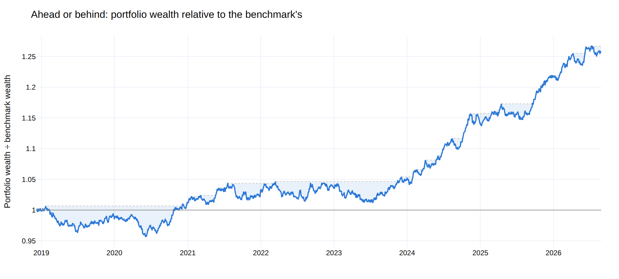
What "3.08% of excess return" felt like to hold is a different question, and the relative wealth curve is the one that answers it. This is the ratio of the two wealth curves, not the compounded excess return — compounding a difference of returns as though it were a return overstates the gap, and the error grows with the sample. The shaded bands are relative drawdown: the stretches during which the portfolio was behind the index it is measured on, which is what a client remembers and what no absolute chart shows.
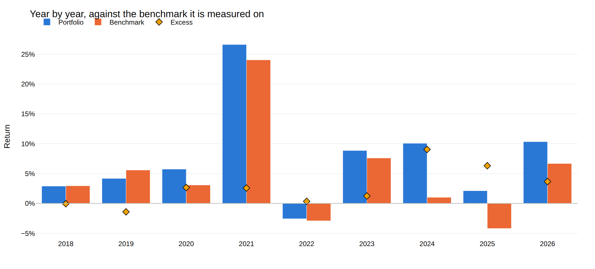
Annualized figures hide the shape of a record, so the same report tabulates it period by period. Here the portfolio beat the index in seven of the nine calendar periods, and the two it lost were the first two — a shape that a single information ratio summarises away, and that decides whether anyone is still invested by the third year.
active_mean_variance goes further and optimizes in active space directly:
maximize α'x − λ·x'Σx over x = w − b, or maximize expected active return
subject to √(x'Σx) ≤ TE* when a budget is set. With b = 0 it reduces
exactly to mean_variance, which is the check that the reformulation is not
quietly a different problem.
Active management (Grinold-Kahn)
For a portfolio measured against a benchmark, the engine computes the pieces of
the fundamental law IR ≈ TC · IC · √BR:
- The information coefficient from a forecast panel, with the t-statistic that says whether the skill is distinguishable from zero.
- The transfer coefficient — how much of the forecast survived the mandate. The engine knows exactly which constraints were applied and what the unconstrained answer would have been, so this is a measurement rather than an estimate. A transfer coefficient of 0.35 says two thirds of the skill is being absorbed by the constraints, which points at a different fix than "get better signals".
- Grinold's alpha,
α = IC · σ · z, which turns a score into a defensible expected return. With an IC of 0.05, a two-standard-deviation view on a 20%-vol asset is worth 2% — not the 10% that gets typed into a spreadsheet, and the difference is exactly what stops mean-variance cornering. - Risk-aversion calibration,
λ_A = IR / (2ψ*): a tracking-error budget and a believed information ratio imply the utility coefficient, rather than it being guessed. - The Euler decomposition of tracking error, which disagrees with the absolute one precisely on the large benchmark positions that carry plenty of risk and no active risk at all.
implied_breadth()run backwards is a plausibility check: an IR of 1.0 on an IC of 0.03 needs 1,111 independent bets a year.
Estimation error
The engine spends a lot of effort saying that expected returns and covariances are noisy — condition numbers, T/N ratios, walk-forward degradation — so it does not then draw the frontier as a single crisp line and leave it there:
-
bootstrap_frontier()resamples the return history (block, IID or parametric), re-estimates and re-traces the frontier on each draw, and returns the resulting confidence band plus the per-asset weight dispersion. On the sample panel the frontier's expected return spans a 6.3-percentage- point band at a typical risk level — differences narrower than that are not distinguishable from noise. -
resampled_efficient_frontier()implements Michaud-style resampling: averaging weights across draws at each frontier rank, which lifts the mean effective N from 3.3 to 5.2 on the sample panel because the optimizer stops acting on differences the data cannot resolve. -
monte_carlo_optimization_selection()asks the prior question: given a universe like this one and a sample this long, which method can be trusted to find the right answer at all? It declares the fittedμandΣto be the truth, draws synthetic histories from them, re-estimates and re-solves on each, and measures how far each method lands from the answer that truth implies (López de Prado, 2019). Over 20 draws on the sample panel:Method Weight RMSE Worst single position nco0.01% 0.01% herc0.02% 0.05% hrp0.05% 0.13% min_variance0.59% 1.51% mean_variance14.79% 35.53% Each method is scored against its own answer on the truth, not a common one — the question is estimation stability, not which objective is right.
Selection bias
Running forty configurations and reporting the best one is easy in a library with ten methods, six covariance estimators and a grid of constraints. The maximum of forty noisy estimates is a biased estimate of the best true value, and nothing about that bias is visible in the number itself.
deflated_sharpe_ratio()(Bailey & López de Prado, 2014) deflates against the expected maximum across the trials you actually ran, adjusted for skew and kurtosis. Take 50 strategies drawn from the same zero-mean distribution: the best posts an annualized Sharpe of 1.24 and a probabilistic Sharpe of 99.3%. Its deflated Sharpe is 45.9%.minimum_track_record_length()says how much history you would need before the observed Sharpe is significant. Usually a bracing answer.probability_of_backtest_overfitting()implements CSCV: across every balanced split of the sample, how often does the in-sample winner land below the out-of-sample median? Above ~50% your selection process is a coin flip.
optengine optimize --trials 40 makes the declaration explicit. The default of
1 is a claim, and the output says so.
Backtesting
The simulation lives in optimization_engine.backtest, organized around one
boundary: a stateless core that turns weights into a track record, and the
layers that judge what came out. The core reads no files, keeps no state
between calls, and is deterministic given its inputs — which is what makes the
diagnostics above meaningful and lets a whole grid be run without the cells
interfering with each other.
BacktestSpec is the declarative description of a run: cadence, cost model,
execution lag, annualization. It is data rather than code, so it serializes,
diffs, and hashes. Two runs carrying the same spec_hash were asked the same
question; result_hash says whether they got the same answer.
from optimization_engine import BacktestSpec, CostSpec, run_backtest

spec = BacktestSpec(
    frequency="monthly",
    costs=CostSpec(commission_bps=8, slippage_bps=4, impact_coefficient=0.4),
    execution_lag=1,          # decide on the close, fill on the next one
)
run = run_backtest(returns, weights, spec)
Three things that in-sample constant-weight replays quietly assume away:
- Drift and rebalancing. Positions grow with their own return between
trades; pulling them back costs money.
run_backtest()reports held weights (not targets), per-trade costs, turnover, and NAV. - Execution.
execution_lagseparates the date a target is chosen from the date it is traded. At zero — the conventional default — the book fills on a close it has not seen. - Cost that scales.
CostSpecsplits commission (a broker problem) from slippage and market impact (a size problem). Withimpact_coefficientset, cost follows the square-root laweta · sigma · sqrt(q / participation), so the same allocation gets more expensive as the book grows — the only way capacity shows up in a backtest at all. When the trailing volatility behind that estimate is missing, the trade degrades to the linear charge and the run says so onmeta.degradationsrather than silently charging zero. A walk-forward hands the cost models the whole history as context, so its first trades are priced off the years that precede them rather than degrading for want of data sitting just outside the evaluation window — only rows strictly before each decision date are ever read.
walk_forward_run() re-estimates and re-solves on a rolling (or expanding)
window and holds each solution forward over returns the optimizer never saw;
a failed solve carries the previous book forward and is recorded, because
skipping the period would delete a real cost from the track record.
compare_in_and_out_of_sample() puts the two track records side by side with
the degradation between them.
The two cadences are separate arguments, because they are separate
decisions. rebalance_every is how often the optimizer re-solves — how stale
the desk is willing to let its view get. rebalance_frequency is how often the
book is traded back to whichever target is current — how far it is willing to
let the weights drift from that view. A quarterly investment committee running
a monthly rebalancing discipline re-solves four times a year and trades twelve,
and tying the two together understates that policy's turnover:
walk = run.walk_forward_run(
    rebalance_every=63,            # re-optimize quarterly (daily panel)
    rebalance_frequency="monthly", # but pull the book back monthly
)
print(walk.n_resolves)      # 4 a year: how often the view was refreshed
print(walk.n_trade_dates)   # 12 a year: how often it was actually traded
rebalance_frequency defaults to "none" — hold each solution untouched until
the next one — so a run only pays for the extra trading when it asks for it.
Passing nothing leaves the trading calendar to the spec's own frequency, and
an explicit argument overrides the spec; nothing is silently discarded either
way. On the command line the pair is --rebalance-every N --rebalance CADENCE.
On top of the core:
-
compute_tca()— the cost panel. A total is uninformative on its own, so it normalizes: cost per unit of traded notional, cost per rebalance, annualized drag, and the commission/impact split. Ratios that cannot be computed come back asNonewith a reason, never as a zero that reads like a measurement.cost_by_asset()says where it went. -
compute_position_stats()— the round trips hiding in the weight path. Every asset's stay in the book is an episode with a contribution and a holding period, so the usual win rate, profit factor and payoff ratio apply. A Sharpe earned by three names is a different risk from the same Sharpe earned by two hundred, and the return curve cannot tell you which one you have. -
run_sweep()— grids, with the discipline that makes them safe.SweepResultscannot represent a partial grid: the invariant is checked on construction, and a cell that fails to build or fails to solve becomes an error row, never a missing one. There is deliberately nobest(), notop_n(), no sort by Sharpe. What it does give you is the trial count — the input the deflated Sharpe and the overfitting probability both need, and the one nobody records.results.deflated_sharpe(cell)andresults.overfitting_report()wire straight into §5 above. -
final_holdout_run()— the segment nothing was fitted on, and the audit log that keeps it that way.gate_returns()physically truncates the history before any run can see it;assert_within_holdout()fails loudly if untruncated data reaches a gated path anyway. Every visit to the held-out segment is appended to a JSONL log, and repeat visits earn flags:REPEATEDfor the same specification seen twice,SHIFTED_HOLDOUTfor the same strategy evaluated against a boundary that moved. The flags block nothing. They make the second look visible, which is all a diagnostic can honestly do.The log is committed —
runs/holdout_audit.jsonlis the one file this repository keeps out of its ownruns/ignore rule. Selection bias accumulates across people as much as across sessions, and a log living on one laptop is a control the controlled party resets by cloning fresh..gitattributesgives it a union merge so concurrent appends never conflict. Since it is published, keep thestrategymapping to identifiers — a config path, a spec hash — rather than a payload. -
build_tearsheet()— the assembled reading. Performance, drawdowns, costs, position statistics and the selection-bias correction in one object, with the caveats attached to the numbers rather than to a footnote. A tearsheet over an in-sample, costless, same-period-fill run says all three things out loud.Expected returns are re-derived inside each window by default (
reestimate_expected_returns=True). This matters more than it sounds:config.expected_returnsis normally populated — the UI seeds that table from the full history — so reusing it would hand every "out-of-sample" window an estimate built partly from its own future. On the sample panel that look-ahead lifts walk-forward Sharpe from 0.46 to 0.89. Turn it off only when your expected returns are genuine forward-looking assumptions rather than estimates from the same data.
How a run flows
flowchart TD
    A0[Provider<br/>yahoo · stooq · fred · fmp · tiingo · file] --> A1{Preflight}
    A1 -->|asks for a field<br/>the provider lacks| A2[Refused before<br/>the network call]
    A1 --> A[Panel + per-identifier log<br/>homogenized column names]
    A --> B{Data quality}
    B -->|gaps, stale feeds,<br/>splits, thin samples| B1[Reported before<br/>anything is estimated]
    B --> C[Align panel<br/>explicitly, with a log]
    C --> D[Covariance<br/>+ conditioning diagnostics]
    C --> E[Expected returns<br/>historical · EMA · CAPM · shrunk]
    D --> F{Feasibility}
    E --> F
    F -->|impossible| F1[Names the constraint<br/>and the fix]
    F -->|solvable| G[Optimize]
    G --> H{Constraints respected?}
    H -->|breach| H1[Reported, never silent]
    H --> I[Weights + diagnostics<br/>effective N · risk decomposition]
    I --> J[Frontier<br/>+ resampled confidence band]
    I --> K[Backtest<br/>drift · costs · walk-forward]
    J --> L[Excel report<br/>carrying its own assumptions]
    K --> L
Layout
src/optimization_engine/
├── analytics/        # performance · risk · relative · backtest (compact API)
│                     # active (Grinold-Kahn) · diversification (Meucci)
│                     # selection (deflated Sharpe · PBO)
├── backtest/         # spec · costs · calendar · runner · results (the core)
│                     # walkforward · tca · positions · sweep · holdout
│                     # tearsheet
├── data/             # loaders · covariance · denoising · data-quality
├── ingest/           # multi-provider spine: one request in, one validated
│                     # panel out, with per-identifier provenance
│   ├── spec · fields · panel · errors      (what a request and a panel are)
│   ├── providers/    # yahoo · stooq · fred · fmp · tiingo · file · sample
│   ├── registry · credentials · catalog    (name → provider → symbol)
│   └── cache · service                     (disk cache, concurrency, run log)
├── optimizers/       # one file per technique + diagnostics + feasibility
├── reporting/        # Excel exporter + Plotly figures
├── benchmark.py      # what the portfolio is measured — and optimized — against
├── config.py         # YAML/JSON-driven config
├── engine.py         # high-level façade (run_engine)
├── frontier.py       # efficient frontier sweep
├── resampling.py     # bootstrap bands · Michaud resampling · MCOS
└── cli.py            # `optengine` entrypoint
app/
├── streamlit_app.py  # interactive UI
├── data_sources.py   # provider picker, ingest log, liquidity selector
└── components.py     # reusable render blocks
config/               # example configs
docs/RESEARCH.md      # the literature behind the methods, and what was left out
docs/images/          # README figures (regenerate with scripts/)
notebooks/            # quickstart notebook
scripts/              # batch runners + docs-figure renderer
tests/                # pytest suite
Install
pip install finport-optengine
That is the core: the optimizers, the covariance estimators, the backtest and the analytics, on numpy, pandas, scipy, cvxpy, scikit-learn and pyyaml. The parts most callers do not need are extras:
| Extra | Pulls | Needed for |
|---|---|---|
viz |
plotly | Every figure in reporting.plots |
excel |
openpyxl, xlsxwriter | Reading and writing .xlsx |
stats |
statsmodels | Benchmark-relative OLS metrics (beta, regression stats) |
mcp |
mcp | The MCP server, optengine-mcp (needs Python 3.10+) |
data |
yfinance, pyarrow | The Yahoo provider, and Parquet panels |
ui |
streamlit, ipywidgets, plotly | The Streamlit app |
all |
everything above except ui and mcp |
The CLI's worked examples |
Reaching a feature whose extra is missing raises with the command that fixes
it, rather than a bare ModuleNotFoundError. To run the CLI end to end:
pip install "finport-optengine[all]"
For a source checkout, working on the engine itself:
pip install -e ".[all,ui,mcp,dev]"
The import name stays optimization_engine and the console script stays
optengine, whichever way it was installed.
Use it
Streamlit UI
streamlit run app/streamlit_app.py
The sidebar walks a numbered path — Data → Currency → Method → Assumptions → Objective → Benchmark → Exposure → Frontier — and each step surfaces what could make the next one wrong.
-
Data — pick a provider, name a universe, fetch. The picker states each provider's capabilities up front and greys out what it cannot serve, so asking FRED for volume is unavailable rather than an error after the fact; a provider needing a key says which variable it reads and lets you paste one for the session. What comes back is shown as a provenance block — which symbol, which provider, which instrument kind, which currency, how many observations, and whether the series carries volume — beside the data-quality report: interior gaps, stale feeds that read to an optimizer as low volatility, unadjusted splits, and how many periods actually have every asset present. The missing-data policy is an explicit choice, and the app logs exactly what it did to the panel.
-
Assets — per-asset statistics (extended metrics on a toggle) plus a drawdown-episode table with peak, trough, recovery and time underwater.
-
Assumptions & constraints — editable expected returns, weight bounds, asset-class budgets, a layered-limit builder where you add as many levels of the mandate as it has (name the buckets, assign assets from a dropdown or fill them in one click from the Group or Currency column, and cap each bucket as a share of the portfolio or of its parent), per-method inputs (risk budgets, Black-Litterman views both absolute and relative, cluster counts and linkage for HERC/NCO, the CDaR tail), the covariance estimator with its denoising and detoning toggles, and a live feasibility check that names the constraint making the problem impossible and what to change, before you ever press solve.
-
Optimize — a compliance banner, KPI cards, concentration and diversification measures, a policy-exposure table that says where the book landed on every layer and marks which bucket actually stopped it, a capital-vs-risk chart, the full Euler decomposition (with risk shares per layer, because a 30% bond sleeve rarely carries 30% of the risk), and a frontier marked with the minimum-variance and tangency portfolios, the capital allocation line, and where your portfolio actually sits — plus an opt-in panel that redraws the frontier as a confidence band and names the positions the sample cannot pin down.
-
Backtest — choose a rebalancing cadence, an execution lag, and a cost model split into commission, spread and square-root market impact, plus where the impact model's participation rate comes from: a fixed assumption, or the traded volume the panel actually carries — with a fund size, because capacity is a currency amount and the same strategy costs more to run at ten times the size. Choosing volume on a universe that has none — every index universe — falls back to the fixed rate and says so on the page rather than in a log; see weight drift, cost drag, where the cost went by name, rolling performance, the return distribution with its VaR/CVaR cuts, and a walk-forward run that says in words how much of the result was hindsight.
-
Performance — absolute and relative on one page, both computed on the same aligned sample: KPI cards for each, cumulative wealth against the benchmark and the relative wealth curve with its underwater band, calendar-period bars, rolling absolute and rolling relative panels, a risk-return scatter placing the portfolio and its benchmark among the assets they are built from, and the full tables. Exports as a workbook or as a tidy metrics CSV.
-
Compare / What-if — saved scenarios side by side, and live re-solving as you drag weight bounds.
-
Report — one-click Excel export carrying assumptions, diagnostics, data-quality findings, the benchmark and active weights, the full performance report and the walk-forward comparison alongside the weights.
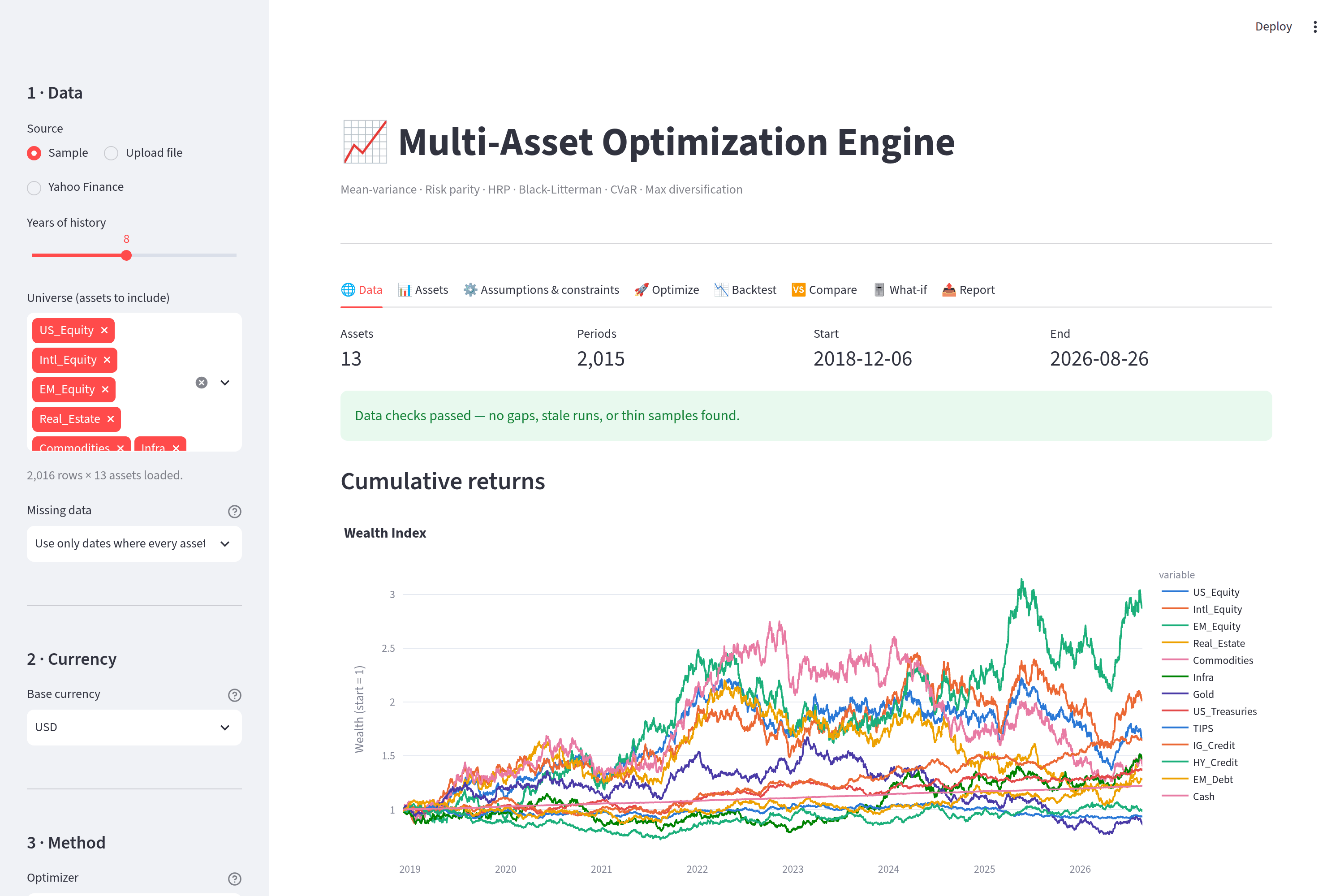
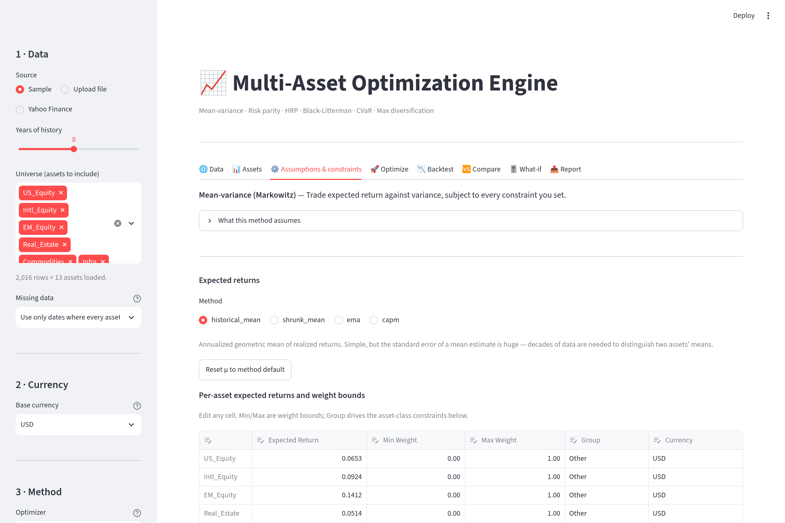
The Benchmark step is one choice that everything downstream reads: the
relative block on the backtest page, the performance page, the workbook, and —
when you set a tracking-error or active-share limit — the solve itself. Any
series you load but leave out of the universe is offered there as an external
benchmark, so pulling ^GSPC alongside your tickers and deselecting it is all
it takes to measure against the index.
The sidebar's 📚 Scenarios block saves, updates, loads, renames, deletes, and downloads/uploads named profiles (YAML).
CLI
optengine list-optimizers                    # each method with a one-line summary
optengine describe hrp                       # what it needs, supports, assumes
optengine providers                          # data sources, capabilities, key status
optengine sample-data --output data/sample/sample_prices.csv

# Fetch a panel. Prices and volume are written separately, because a universe
# can perfectly well have the first and not the second.
optengine ingest --provider yahoo --identifiers "SPY,EFA,EEM,AGG,GLD" \
    --ingest-period 10y --ingest-fields ohlcv \
    --output prices.parquet --volume-output volume.parquet

# The same universe from a different provider. Nothing else changes: catalog
# names resolve to each provider's own symbol and the columns keep their names.
optengine ingest --provider stooq --identifiers "SP500,DAX,IPC" \
    --ingest-period 10y --output indices.csv

# Optimize straight off a provider, with a disk cache so a re-run does not
# re-download.
optengine optimize --config config/example_multi_asset.yaml \
    --provider yahoo --identifiers "SPY,EFA,EEM,AGG,TLT,GLD,DBC,VNQ" \
    --ingest-period 10y --ingest-currency USD --cache-dir .cache/panels

# Pre-flight the inputs and constraints without solving.
optengine check --config config/example_multi_asset.yaml --sample

# Solve, and refuse rather than fail obscurely if the mandate is impossible.
optengine optimize --config config/example_multi_asset.yaml --sample \
    --frontier --resample 50 --walk-forward --cost-bps 10 --strict

# Filter the covariance's noise eigenvalues, declare how many configurations
# you tried, and rank the methods by how reliably each recovers the truth.
optengine optimize --config config/example_multi_asset.yaml --sample \
    --denoise --walk-forward --trials 40 --mcos 20

# Measure against a benchmark, and hold the solve to an active-risk budget.
# --benchmark takes a kind ('equal_weight'), an asset name, or 'none' to
# override whatever the config's benchmark block says.
optengine optimize --config config/example_multi_asset.yaml --sample \
    --benchmark equal_weight --max-tracking-error 0.03 --max-active-share 0.5

# Walk the process forward, price the trading properly, and count the trials.
# --execution-lag defaults to 1: a desk does not trade on a close it has not
# seen. Every sweep cell is walk-forwarded, and its trial count is carried into
# the deflated Sharpe rather than left for the reader to guess.
optengine backtest --config config/example_multi_asset.yaml --sample \
    --commission-bps 8 --slippage-bps 4 --impact-eta 0.4 \
    --sweep optimizer.name=min_variance,risk_parity,equal_weight \
    --output backtest.xlsx

# Withhold everything after a date, walk forward on the rest, then look at the
# held-out segment once — and write that look down.
optengine backtest --config config/example_multi_asset.yaml --sample \
    --commission-bps 10 --holdout 2024-01-01

# Price capacity from real traded volume rather than an assumed participation
# rate. Costs now rise as the fund grows and as a name's turnover dries up —
# which is why --initial-capital becomes mandatory here: capacity is a
# currency amount, so a run that does not state a fund size is refused rather
# than reporting a cost of roughly zero.
optengine backtest --config config/example_multi_asset.yaml \
    --provider yahoo --identifiers "SPY,EFA,EEM,AGG,GLD" \
    --ingest-period 10y --ingest-fields ohlcv \
    --impact-eta 0.4 --impact-participation-source adv \
    --impact-adv-share 0.10 --initial-capital 250000000

# The same run on an index universe, which has no volume and never will. It
# does not fail: impact falls back to the fixed participation rate, and every
# trade that did so is named in the run's degradation notes.
optengine backtest --config config/indices.yaml \
    --provider stooq --identifiers "SP500,DAX,NIKKEI225,FTSE100" \
    --ingest-period 10y --impact-eta 0.4 \
    --impact-participation-source adv --initial-capital 250000000
backtest prints what the strategy earned out of sample, what the trading cost
to get it, and how much of the remaining Sharpe survives being deflated for the
size of the search. It ends with the caveats the run did not answer — costs
not modelled, orders filled on a price nobody could have traded at, a Sharpe
nobody deflated. A second visit to the same holdout comes back flagged
REPEATED; the same strategy against a boundary that moved comes back
SHIFTED_HOLDOUT.
A benchmarked run prints the relative headline alongside the absolute one, and
the workbook gains the benchmark, the active weights, and the full absolute
and relative performance report — plus the same report on the walk-forward
returns when --walk-forward is set, so the fitted information ratio sits
next to the out-of-sample one.
check exits non-zero when the data has errors or the constraints have no
solution, so it drops straight into CI or a pre-commit hook.
Four commands take --json: optimize, backtest, check and describe.
Human narration moves to stderr, so stdout is exactly one parseable document
and a pipeline can act on a result without scraping a formatted table.
optengine describe risk_parity --json | jq '{name, requires, supports}'
{
  "name": "risk_parity",
  "requires": {
    "expected_returns": false,
    "covariance": true,
    "return_history": false,
    "benchmark": false
  },
  "supports": {
    "target_return": false,
    "target_volatility": false,
    "risk_aversion": false,
    "risk_free_rate": false,
    "group_bounds": true,
    "frontier": false,
    "turnover": false,
    "benchmark_limits": false
  }
}
Read describe --json before building a config. supports.turnover false
means a turnover budget is ignored, not rejected, and nothing will tell you
at runtime.
Every payload carries schema_version, so a consumer can refuse a major it
does not know. A command that fails still emits JSON — an object with error
and exit_code — whether it returned a code or raised, so a caller never has
to distinguish "no output" from "output I could not parse". The builders are
importable at optimization_engine.reporting.payloads if you are in-process
rather than shelling out.
MCP server
For agents that call tools rather than write code. optengine-mcp speaks the
Model Context Protocol over stdio.
pip install "finport-optengine[mcp]"   # needs Python 3.10+
optengine-mcp                          # speaks stdio; narration on stderr
Register it by pointing a client at the console script. Claude Code takes it from the command line:
claude mcp add optimization-engine -- optengine-mcp
Any client reading a JSON config — Claude Desktop's
claude_desktop_config.json, and most others — takes the same server as:
{
  "mcpServers": {
    "optimization-engine": {
      "command": "optengine-mcp"
    }
  }
}
If the client cannot see your PATH, give the absolute path to the script
instead — /path/to/venv/bin/optengine-mcp.
Five tools:
| Tool | What it answers |
|---|---|
list_optimizers |
Which methods exist, one line each. Start here when you don't yet know what a mandate needs |
describe_optimizer |
What one method requires as input, and which constraints it will actually honour |
check_mandate |
Can these constraints be satisfied at all; what return range is reachable; is the covariance conditioned well enough to optimize on |
optimize |
Weights, plus which solver answered, whether the constraints held, and how concentrated the book is in risk rather than capital |
backtest |
The process walked forward with commission, slippage and market impact, plus the hashes that identify the run |
They return the same payloads as --json, built by the same module, so the
two surfaces cannot drift apart. Pass sample: true for the built-in panel or
prices_path for a file of prices; config_path takes the same YAML the CLI
reads.
Three of the five read filesystem paths — config_path and prices_path.
None writes a file, fetches over the network, or touches a keyed provider. Solving blocks — a large solve is seconds of CPU
and these tools are synchronous, so a client that looks hung is usually an
optimizer working.
Failures a tool anticipates come back with their message intact; anything
unanticipated is wrapped by the SDK as Error executing tool optimize with
the reason discarded, which is why every reachable bad-input path raises the
SDK's own error type.
Python
from optimization_engine import (
    EngineConfig, OptimizerSpec, run_engine,
    sample_dataset, prices_to_returns, analyze_prices,
)

prices = sample_dataset()
print(analyze_prices(prices).describe())

returns = prices_to_returns(prices)

config = EngineConfig(
    expected_returns={c: 0.05 for c in returns.columns},
    bounds={c: [0.0, 0.4] for c in returns.columns},
    optimizer=OptimizerSpec(name="risk_parity"),
)

run = run_engine(returns, config, build_frontier=True)
print(run.result.weights.round(3))
print(run.result.violations)          # empty when fully compliant
print(run.diagnostics.effective_n)    # concentration, not just position count
print(run.risk_decomposition())       # contributions in volatility units

# What survives out of sample?
wf = run.walk_forward(transaction_cost_bps=10)
print(run.in_vs_out_of_sample(wf))

# Measured against what? State it once, and both the report and the solve
# read the same answer.
from dataclasses import replace

from optimization_engine import BenchmarkSpec

relative = replace(
    config,
    optimizer=OptimizerSpec(name="mean_variance", risk_aversion=3.0),
    benchmark=BenchmarkSpec(kind="equal_weight"),
    max_tracking_error=0.03,          # binds inside the mean-variance solve
)
relative_run = run_engine(returns, relative)

report = relative_run.performance(frequency="monthly", transaction_cost_bps=10)
print(report.describe())              # one paragraph, hedged where it should be
print(report.relative.T)              # excess, T.E., IR, alpha and its t-stat,
                                      # capture, batting average, M², …
print(report.periods)                 # portfolio vs benchmark, year by year
report.metrics().to_csv("metrics.csv", index=False)   # tidy, diffable

# The same report, on returns this process never saw. Its own walk-forward,
# not the one above — that belonged to a different config.
relative_wf = relative_run.walk_forward(transaction_cost_bps=10)
print(relative_run.performance(returns_override=relative_wf.returns).describe())

# ...and how much of *that* is the forty configurations you tried first?
from optimization_engine import deflated_sharpe_ratio
print(deflated_sharpe_ratio(wf.returns, n_trials=40).describe())

# The full simulation stack: a validated spec, real execution, real costs.
from optimization_engine import BacktestSpec, CostSpec, SweepSpec

spec = BacktestSpec(
    frequency="monthly",              # the trading calendar, honoured as written
    costs=CostSpec(commission_bps=8, slippage_bps=4, impact_coefficient=0.4),
    execution_lag=1,
)
walk = run.walk_forward_run(spec=spec, rebalance_every=63)
print(walk.describe())                # re-solves vs. trade dates, side by side
print(walk.run.meta.result_hash)      # same spec + same data => same hash
print(walk.run.trades.head())         # per-asset fills with the cost split
print(walk.weight_stability())        # is the optimizer chasing noise?

# Don't guess the trial count — run the grid and let it count itself.
sweep = run.sweep(SweepSpec(params={
    "optimizer.name": ["min_variance", "risk_parity", "equal_weight"],
    "covariance_method": ["sample", "ledoit_wolf"],
}))
print(sweep.describe())               # every cell, failures included
print(sweep.overfitting_report().describe())
print(sweep.deflated_sharpe(0).describe())

# One object with the numbers and the caveats attached to them.
sheet = run.tearsheet(walk.run, n_trials=sweep.n_ok,
                      trial_sharpes=sweep.trial_sharpes())
print(sheet.describe())
print(sheet.tca.to_frame())           # cost per notional, per trip, per year
print(sheet.positions.to_frame())     # win rate and holding period by position

# How many bets is this, once correlations are accounted for?
print(run.diversification_comparison())
Layered constraints
A mandate is written in levels, and a single flat grouping can only express
one of them. constraint_layers takes as many as the policy has; all of them
bind at once.
from optimization_engine import (
    EngineConfig, OptimizerSpec, currency_layer, layer_from_mapping, run_engine,
)

asset_class = {"SPY": "Equity", "EFA": "Equity", "EEM": "Equity",
               "AGG": "Fixed Income", "EMB": "Fixed Income", "GLD": "Commodities"}

config = EngineConfig(
    expected_returns=mu,
    # Layer 1: no more than 60% equity, 30% fixed income, 10% commodities.
    groups=asset_class,
    group_bounds={"Equity": [0.0, 0.60],
                  "Fixed Income": [0.0, 0.30],
                  "Commodities": [0.0, 0.10]},
    constraint_layers=[
        # Layer 2: inside equity, at most 30% emerging — of the *sleeve*, so
        # the cap moves with whatever the optimizer puts in equity. The parent
        # bucket of each child is derived from the assignments, not typed twice.
        layer_from_mapping(
            "Sub-asset class",
            {"SPY": "DM", "EFA": "DM", "EEM": "EM", "AGG": "DM FI", "EMB": "EM FI"},
            {"EM": 0.30, "EM FI": 0.25},
            basis="parent", parent="Asset class",
        ),
        # Layer 3: at most 30% foreign currency, cutting across both.
        currency_layer(
            "FX exposure",
            {"SPY": "USD", "EFA": "EUR", "EEM": "EUR",
             "AGG": "USD", "EMB": "USD", "GLD": "EUR"},
            base_currency="USD", foreign_max=0.30,
        ),
    ],
    optimizer=OptimizerSpec(name="max_sharpe"),
)

run = run_engine(returns, config)
print(run.layer_exposures())            # every bucket, its limit, its headroom
print(run.layer_risk_contributions("Sub-asset class"))   # risk, not capital
layer_exposures() restates a percent-of-parent limit as a share of the book
— a 30% cap on a 55% equity sleeve is a 16.5% cap on the portfolio — and marks
the buckets that are binding, which is the answer to "why this portfolio": a
book held at 60% equity by the asset-class cap is a different portfolio from
one held there because the emerging sub-limit ran out.
Every method honours every layer. The convex solves impose them directly; the allocate-then-constrain methods project onto the closest feasible allocation and report the distance. A percent-of-parent limit is homogeneous of degree one, so it survives the change of variables in max-Sharpe and max-diversification rather than being applied afterwards.
Before solving, analyze_feasibility checks each layer's arithmetic and says
what to change — caps that cannot fund a full book, a bucket with limits and
no members, sub-limits that cannot fill the sleeve they sit in, or a bucket
whose members straddle two parents (where "40% of the parent" has no meaning
and the engine refuses rather than guessing).
Which method should you even be using? Measure it rather than argue about it:
from optimization_engine import monte_carlo_optimization_selection

selection = monte_carlo_optimization_selection(
    returns, config,
    methods=("mean_variance", "min_variance", "hrp", "herc", "nco"),
    n_simulations=20,
)
print(selection.describe())
print(selection.ranking())
For a benchmark-relative mandate, the Grinold-Kahn diagnostics:
from optimization_engine import fundamental_law, grinold_alpha

config.benchmark_weights = {c: 1 / len(returns.columns) for c in returns.columns}
run = run_engine(returns, config)

# Needs an expected-return vector that actually varies across assets — a flat
# one carries no cross-sectional view, and the engine says so rather than
# returning a NaN you find out about later.
tc = run.transfer_coefficient()               # how much survived the mandate
print(fundamental_law(0.05, breadth=200, transfer_coefficient=tc).describe())
print(run.active_risk_decomposition())        # tracking error, not total risk

# Turn scores into expected returns you can defend. `scores` is your own
# cross-sectionally z-scored forecast; `residual_vol` is per-asset volatility.
alphas = grinold_alpha(scores, residual_vol, information_coefficient=0.05)
Relative (spread) Black-Litterman views:
from optimization_engine import View

config.optimizer.name = "black_litterman"
config.optimizer.bl_views = [
    View({"US_Equity": 1.0, "EM_Equity": -1.0}, 0.03, label="US over EM"),
]
Note that Black-Litterman optimizes against its equilibrium posterior,
which normally sits well below historical means — a return target that suits
mean-variance is often unreachable here. run_engine checks the target
against the posterior and says so.
Tests
pytest -q
ruff check src app tests scripts
The README figures are regenerated with:
python scripts/render_docs_images.py
The suite covers the covariance estimators and their PSD repair, every optimizer, frontier monotonicity and reachability, ERC properties, Black-Litterman blending with absolute and relative views, constraint compliance, feasibility diagnosis, backtest drift/costs, walk-forward look-ahead safety, data-quality detection, and the CLI's exit codes.
The methods added in 0.3 are tested against the claims that justify them, not just for smoke: that the Marchenko-Pastur fit recovers a known number of planted factors and improves conditioning while leaving the dominant eigenvector alone; that the cluster search recovers a known block structure; that NCO's weights move less than a direct solve's between two halves of the same generated history; that mean-CDaR beats equal weight on realized maximum drawdown; that the deflated Sharpe rejects the best of fifty skill-free strategies while the probabilistic Sharpe accepts it; that the transfer coefficient is exactly 1 for the unconstrained optimum, −1 for its negative, and invariant to gearing; and that the minimum-torsion factors are uncorrelated to machine precision.
The simulation stack is held to its own claims rather than to smoke: that a run
is reproducible — same spec and same data, same result hash — and that a
different cost model produces a different one; that an execution lag actually
leaves the book in cash until the order fills, and that an order which cannot
fill inside the sample never fills at all; that square-root impact charges
three times the rate for nine times the trade, and degrades loudly when the
volatility behind it is missing; that a cost ratio which cannot be computed
comes back as None with a reason rather than a zero; that a grid keeps its
failed cells as rows, so its trial count stays honest; and that a second visit
to the same holdout is flagged REPEATED while a boundary that moved is
flagged SHIFTED_HOLDOUT.
Where the methods come from
docs/RESEARCH.md is the reading behind these methods: what
López de Prado, Cajas, Grinold & Kahn, Meucci, Raffinot and the rest actually
claim, which of it this engine implements, and — the part usually left out —
which of it was read and deliberately deferred, with the reason. If you want to
know why there is no EVaR here yet, that is where it says so.
License
MIT — see LICENSE.
1 maintainer

Metadata
1 maintainer
Release files for finport-optengine 0.5.1
For a detailed explanation of source distributions (sdists) and built distributions (wheels), please see the package formats documentation.
Source distribution (sdist)
| File | Size | Uploaded | Provenance | |
|---|---|---|---|---|
| finport_optengine-0.5.1.tar.gz | 463.6 kB | With provenance | Details |
Built distribution (wheel)
| File | Interpreter | ABI | Platform | Reset |
|---|---|---|---|---|
| finport_optengine-0.5.1-py3-none-any.whl | Python 3 | none | any | Details |
Total release size: 844.4 kB
Release files / finport_optengine-0.5.1.tar.gz
| Download URL | finport_optengine-0.5.1.tar.gz |
|---|---|
| Size | 463.6 kB |
| Tags | Source |
|
SHA-256 checksum How to use checksums |
e1a502f0b66b7f7c85d6f3f8f0d84febb2d3410a6b52cd5e9ec60ae0a0434dad
|
|
BLAKE2b-256 checksum How to use checksums |
64e81c919c9d6c21a5c3318078a72cbd448174e6519f0a04e914938d33e150f2
|
| Upload date | |
|
Uploaded using Trusted Publishing? What is trusted publishing? |
Yes |
| Uploaded via |
twine/7.0.0 CPython/3.13.14
|
Provenance
Provenance describes where a file came from. On PyPI, provenance is shared via attestations, which provide a verifiable record of the build or publishing details. View details, limitations and caveats.


PyPI Publish Attestation
PyPI verified that this artifact, at this checksum, originated from the publisher listed below.
Signed by GitHub Actions, verified by PyPI on Aug 31, 2026.
Transparency logRelease files / finport_optengine-0.5.1-py3-none-any.whl
| Download URL | finport_optengine-0.5.1-py3-none-any.whl |
|---|---|
| Size | 380.8 kB |
| Tags | Python 3 |
|
SHA-256 checksum How to use checksums |
9027cf8618c2ce21f9605205bc940175cf785a42db11a44e9e91c84b2a0fcb79
|
|
BLAKE2b-256 checksum How to use checksums |
43af4ca5f8ee0a3597f6db2634312c94c7579e66fcb6df3a9facb6eff8d2f6b4
|
| Upload date | |
|
Uploaded using Trusted Publishing? What is trusted publishing? |
Yes |
| Uploaded via |
twine/7.0.0 CPython/3.13.14
|
Provenance
Provenance describes where a file came from. On PyPI, provenance is shared via attestations, which provide a verifiable record of the build or publishing details. View details, limitations and caveats.
PyPI Publish Attestation
PyPI verified that this artifact, at this checksum, originated from the publisher listed below.
Signed by GitHub Actions, verified by PyPI on Aug 31, 2026.
Transparency logSecurity for finport-optengine 0.5.1
Provenance
Provenance describes where a file came from. On PyPI, provenance is shared via attestations, which provide a verifiable record of the build or publishing details. View details, limitations and caveats.
Full provenance
All 2 files in this release have been uploaded with provenance metadata.
Attestation for finport_optengine-0.5.1.tar.gz
PyPI Publish Attestation
PyPI verified that this artifact, at this checksum, originated from the publisher listed below.
Signed by GitHub Actions, verified by PyPI on Aug 31, 2026.
Transparency logA note on package security
PyPI is a repository for distributing packages, not a service for auditing them. While third-party security researchers and our staff do their best to detect and remove malicious packages, PyPI cannot guarantee the quality, security or suitability of any given package.
To learn more about protecting yourself from malicious actors, visit our package security documentation.














