

Flow-based generative models for forward and inverse PDE problems.




Documentation · Installation · Quickstart · API reference · Project report
FlowPDE is a PyTorch library for learning conditional distributions between PDE fields. It combines flow matching with neural ODEs to solve forward problems and inverse problems.
What is included
- Poisson, Burgers, and Darcy dataset generation through Exponax
- Forward and inverse datasets, including noisy and partial observations
- Flow matching and maximum-likelihood objectives over the same
NeuralODEFlow - MLP, ConvNet, ResNet, and UNet backbone neural network models
- ODE sampling, EMA training, evaluation in physical units, and reflow
Each of the six problem settings is drawn out under Problem settings.
Installation
FlowPDE requires Python 3.11 or newer.
pip install "flowpde[data]"   # library + Exponax/JAX PDE data generators
pip install flowpde           # library only (bring your own data)
The core install covers the flows, objectives, models, solvers, trainer, metrics and
FieldNormalizer. The data extra adds JAX and Exponax, which the Poisson, Burgers
and Darcy generators in flowpde.datasets need.
From source
With uv, which installs the versions recorded in uv.lock
together with the development tools:
git clone https://github.com/sarperyn/FlowPDE.git
cd FlowPDE
uv sync
source .venv/bin/activate
With pip:
git clone https://github.com/sarperyn/FlowPDE.git
cd FlowPDE
python3 -m venv .venv               # any Python 3.11+
source .venv/bin/activate
python -m pip install -e ".[data]"
For CUDA/JAX and the optional dependencies, see the installation guide.
Quick Example
import torch
from torch.utils.data import DataLoader

from flowpde import NeuralODEFlow, FlowMatchingObjective, Trainer, UNet
from flowpde.datasets import PoissonGenerator, FieldNormalizer

# Generate and normalize f -> u training pairs.
generator = PoissonGenerator(num_spatial_dims=2, num_points=64, domain_extent=10.0)
train_ds = generator.generate(num_samples=1000, seed=42, problem="forward")

normalizer = FieldNormalizer.from_dataset(train_ds)
train_ds.set_normalizer(normalizer)
loader = DataLoader(train_ds, batch_size=32, shuffle=True)

# The flow defines the dynamics; the objective defines how they are trained.
model = UNet(spatial_dim=2, spatial_size=64, base_channels=64)
flow = NeuralODEFlow(model, target_key="target", condition_key="input")
objective = FlowMatchingObjective(flow, path="linear", time_sampler="uniform")

optimizer = torch.optim.Adam(objective.parameters(), lr=1e-4)
trainer = Trainer(objective, optimizer, device="cpu", ema_decay=0.999)
trainer.train(loader, epochs=100, print_stats_interval=10,
              save_dir="results/poisson/", save_interval=25)

# Generate a solution conditioned on a PDE input.
batch = next(iter(loader))
samples = objective.sample(batch["input"], n_steps=50).view_as(batch["target"])
The full quickstart adds validation, checkpointing, and evaluation in physical units.
Notebooks
Six runnable notebooks in notebooks/ pick up where the snippet above
stops:
- Dataset exploration —
poisson_dataset.ipynb,burgers_dataset.ipynb,darcy_dataset.ipynb: generate a dataset, report its field statistics, and plot samples — the quickest way to see what the flow is being asked to learn. - End to end —
poisson.ipynb,burgers.ipynb,darcy.ipynb: generate data, build the flow, train it, and sample conditioned solutions.
The lockfile installs the kernel but not a Jupyter front-end, so either open the files directly in an editor that renders notebooks, or bring one along for the run:
uv run --with jupyterlab jupyter lab notebooks/    # uv
pip install jupyterlab && jupyter lab notebooks/   # activated virtualenv
Problem settings
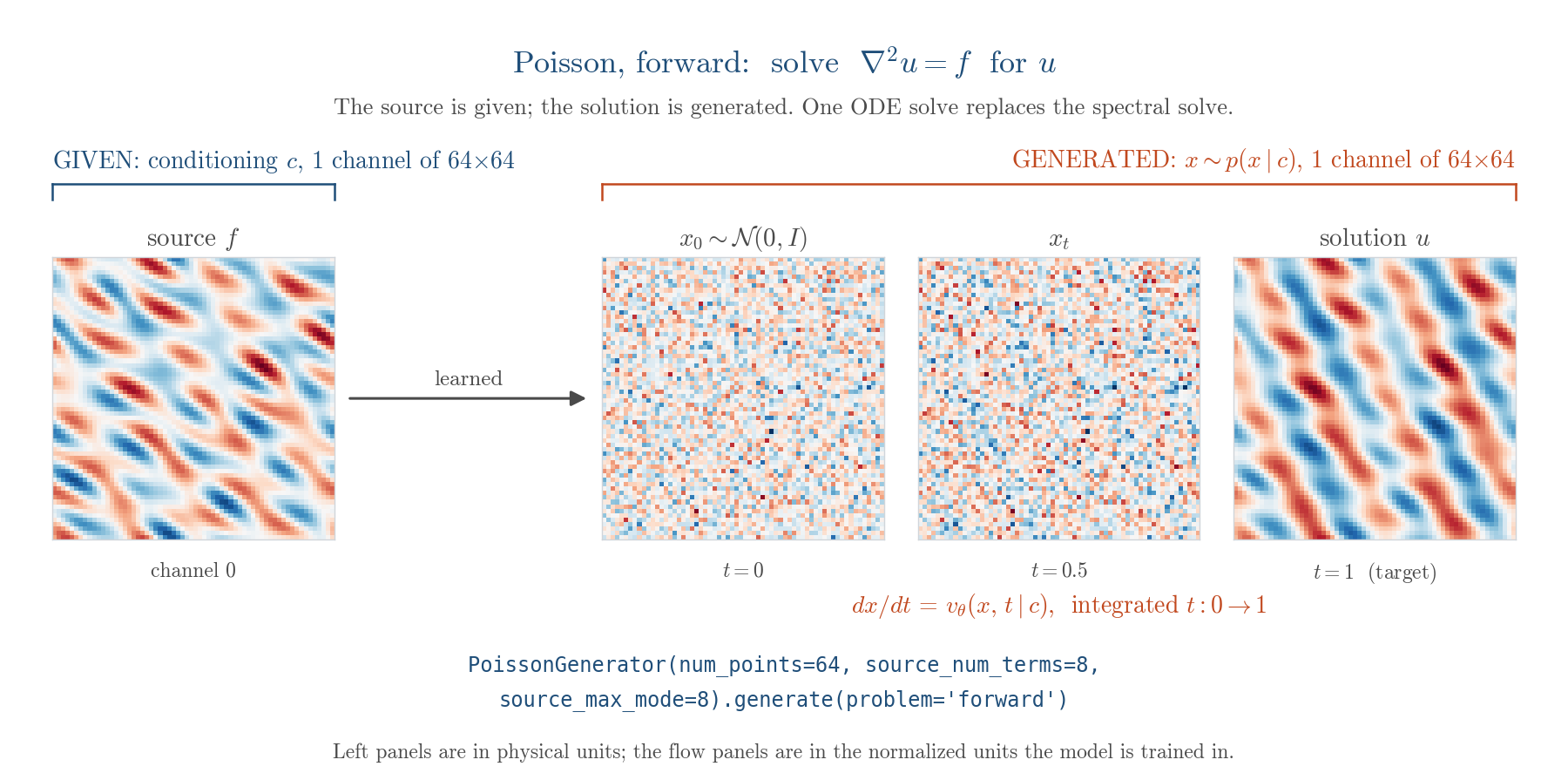
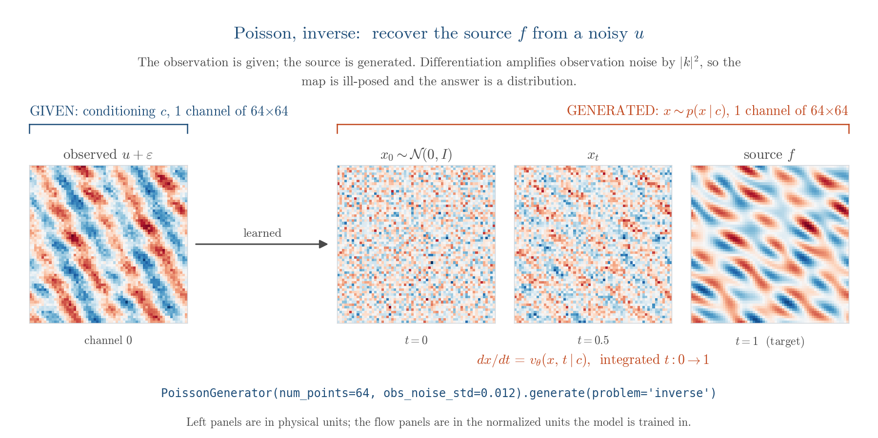
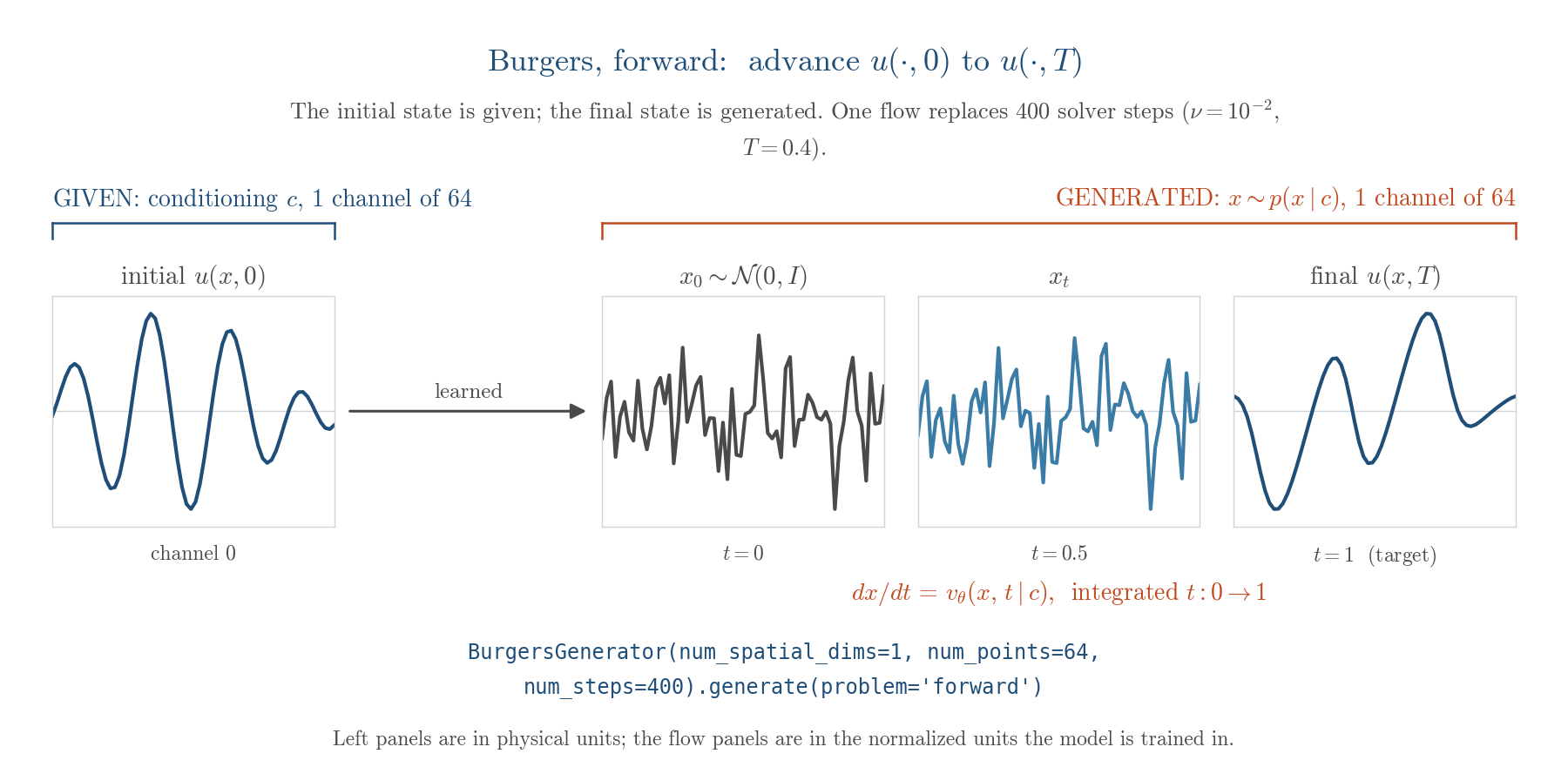
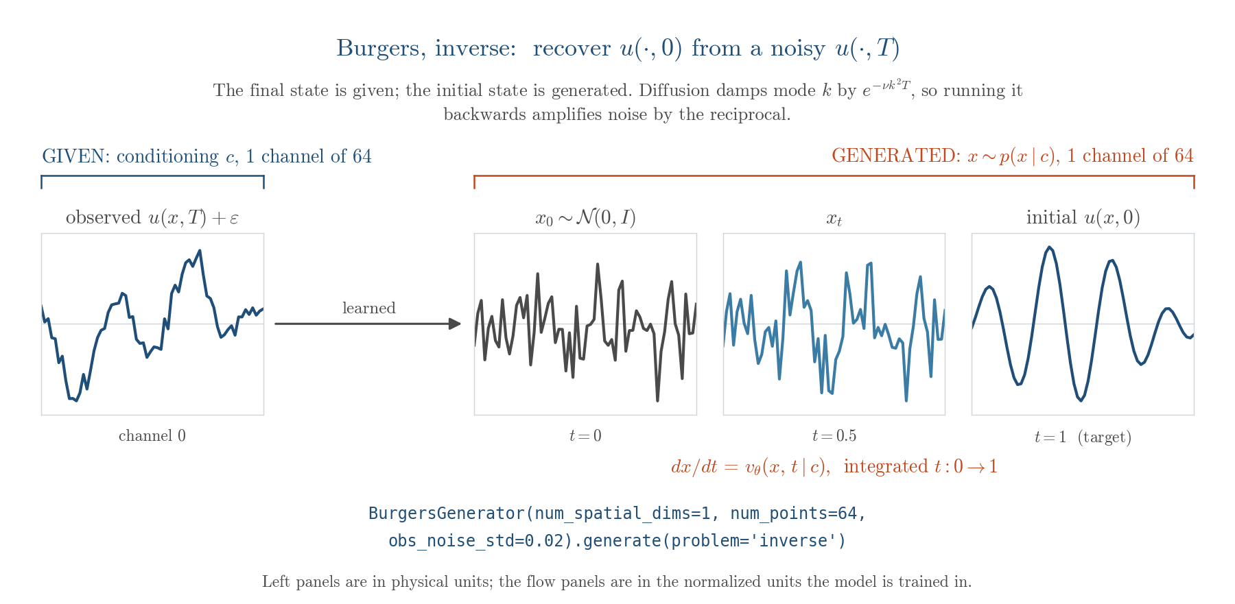
Every PDE is available in both directions: problem='forward' and problem='inverse'
are arguments on the same generator, and all six settings are trained as the same
conditional flow. What changes between them is which fields are handed to the model as
conditioning and which field it has to generate.
Each figure below reads the same way. The left zone is the conditioning input $c$, channel by channel. The right zone is the probability path the flow transports: a draw from the base distribution at $t=0$, the interpolant at $t=0.5$, and the target at $t=1$. What is learned is the velocity field $v_\theta(x, t \mid c)$ connecting them, and sampling is one ODE solve. The footer of each figure is the generator call that produced the fields shown.
Poisson — $\nabla^2 u = f$
Burgers — $\partial_t u + u \partial_x u = \nu \partial_x^2 u$
Darcy — $-\nabla \cdot (\kappa \nabla u) = f$
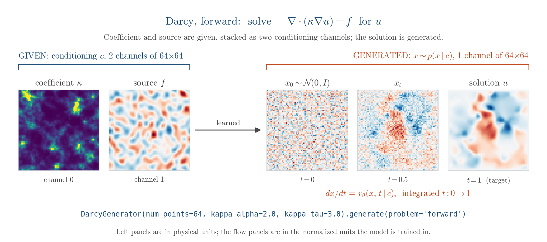
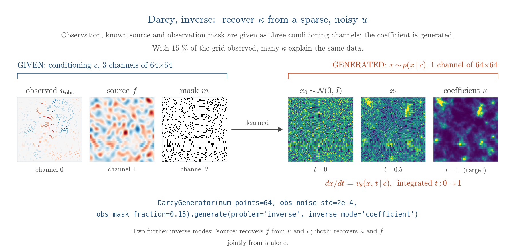
The Darcy inverse problem has three variants, selected with inverse_mode: recover the
coefficient $\kappa$ from $(u, f)$, recover the source $f$ from $(u, \kappa)$, or
recover both jointly from $u$ alone. Observations are degraded independently of the
direction — obs_noise_std adds Gaussian noise, and obs_mask_fraction is the
fraction of grid points that stay observed: anything below 1.0 zeroes out the rest
and appends the observation mask as an extra conditioning channel.
Results
Every comparison below varies one axis with everything else held fixed — data, splits, normalization, optimizer, schedule, averaging, sampler and evaluation seed — so a difference between two numbers is attributable to the thing being varied. Errors are relative $L^2$ in physical units on a held-out test split.
Forward problems
The forward direction is reported as verification rather than as the case for the method. Timed against the conjugate-gradient solver it replaces, the surrogate is 1.9× slower at its cheapest setting and 101× at the setting the accuracy numbers use; on a linear elliptic problem at this size it does not pay for itself.
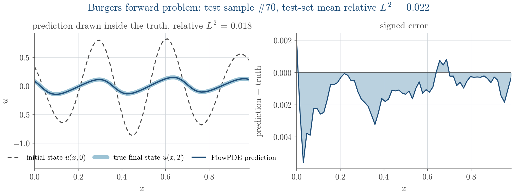
For 1D Burgers, the map from an initial state $u(x,0)$ to the evolved state $u(x,T)$ reaches a test relative $L^2$ of 0.021 with a ConvNet backbone.
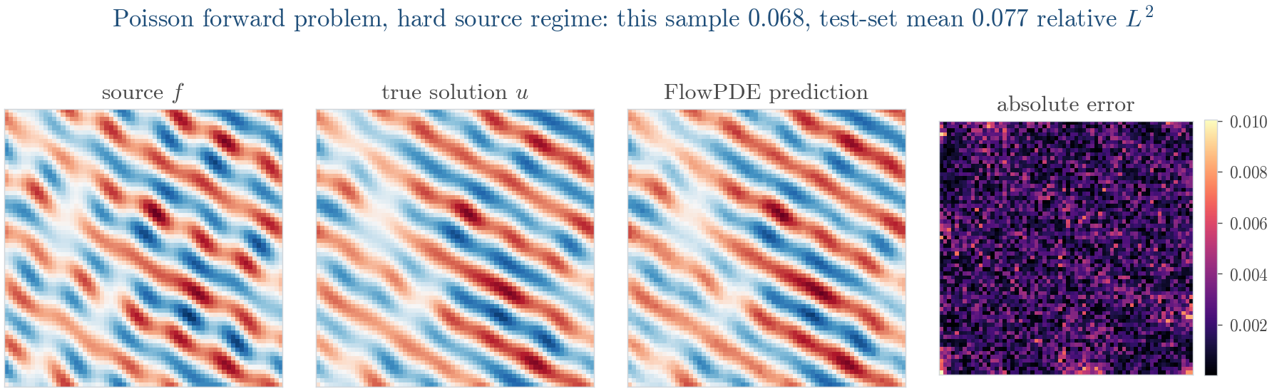
For 2D Poisson, mapping a source $f$ to its solution $u$ in the harder eight-mode source regime reaches 0.078. Widening the source spectrum alone raises the ConvNet's error by 43% — an operator-learning number is a joint statement about the method and the distribution it was measured on, so the harder regime is the one quoted here.
What else the experiments found
- Conditioning. Replacing the conditioner with one that discards its input costs a factor of 17 in median relative $L^2$ while leaving the training loss curve looking healthy — the concrete case for selecting on sampled error, never on the loss.
- Backbone. The smallest of four backbones is the most accurate on Burgers and Darcy, by 12.4× on Burgers, and attention changes nothing beyond seed noise. Capacity is not the binding constraint at this scale. The ordering reverses in one place only, on the widened Poisson source, where the UNet wins by 15%.
- Objective. Fitting the same flow by exact maximum likelihood rather than flow matching improves test likelihood from $-1.21$ to $-1.86$ nats/dim while degrading sample accuracy from 0.61 to 1.06 relative $L^2$, at 70× the wall-clock and 8.9× the memory. Each objective wins on the metric it optimizes.
- Components. Logit-normal time sampling cuts trajectory straightness from 8.17 to 3.70 and is 22% better at two to four evaluations, but 31% worse once the budget is adequate; minibatch-OT coupling straightened the interpolant and not the trajectories, and did not pay at any budget.
- Amortization. A preconditioned Crank–Nicolson reference chain had not mixed after 52,000 forward solves per observation, costing 701 s per observation and producing nothing usable; the trained flow produced its 32-member ensemble in 16 s and needed no forward solves at all. On the smaller Burgers problem where the chain does converge the comparison runs the other way — pCN is five to ten times more accurate and the flow's posterior 6.6–11.1× too wide — but training is paid once, and at 76 s per observation against the flow's 4.0 the two break even after ten inversions.
About the experimentations done using this library; the flow, objective, conditioner, backbone and solver are orthogonal components rather than dependent objects into each other and, thus, every comparison above was a configuration change and this design choice clearly made easier to experiment with different configurations.
Full setup, ablations, and the negative results are in the project report.
The sampler
Solver and step count are call-time arguments on frozen weights, so the whole runs without retraining anything.
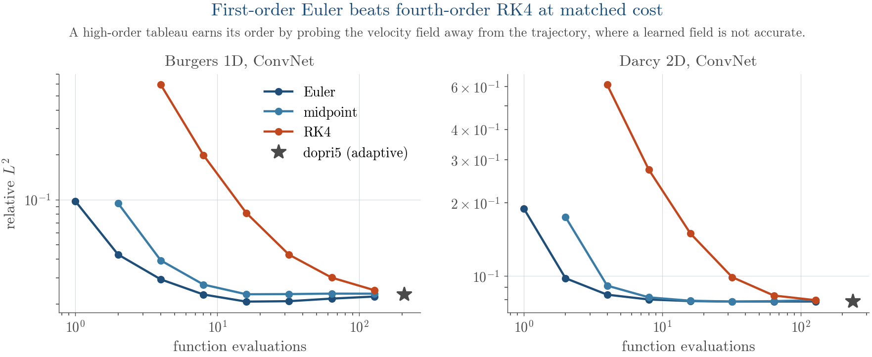
First-order Euler performs better than fourth-order Runge–Kutta when both use the same computational cost, for every model and both problems, with improvements of up to 8.6×. Higher-order methods such as Runge–Kutta evaluate the learned velocity field at extra points away from the actual trajectory, where the model may be less accurate. Also, integrating until full convergence does not always give the smallest error. For two of the eight models, the best fixed-step result has 6–11% lower error than the converged result. This happens because the numerical integration error can partly cancel the model error. Therefore, reporting accuracy only “at 50 steps” can be misleading, since the error does not always decrease as the number of steps increases and the behavior depends on the model.
Tests
The suite covers the flow, the objectives, the solvers, EMA, normalization, reflow,
straightness, and the UQ metrics, plus integration tests that generate real datasets
through Exponax. Those are marked slow because they run the PDE solvers.
uv sync                             # installs pytest and ruff with the dev group

uv run -m pytest                    # full suite
uv run -m pytest -m "not slow"      # skip the Exponax integration tests
uv run -m pytest tests/test_trainer.py -v
In an activated virtualenv, install the test dependencies with
pip install -e ".[data]" pytest and drop the uv run prefix — python -m pytest -m "not slow".
Documentation
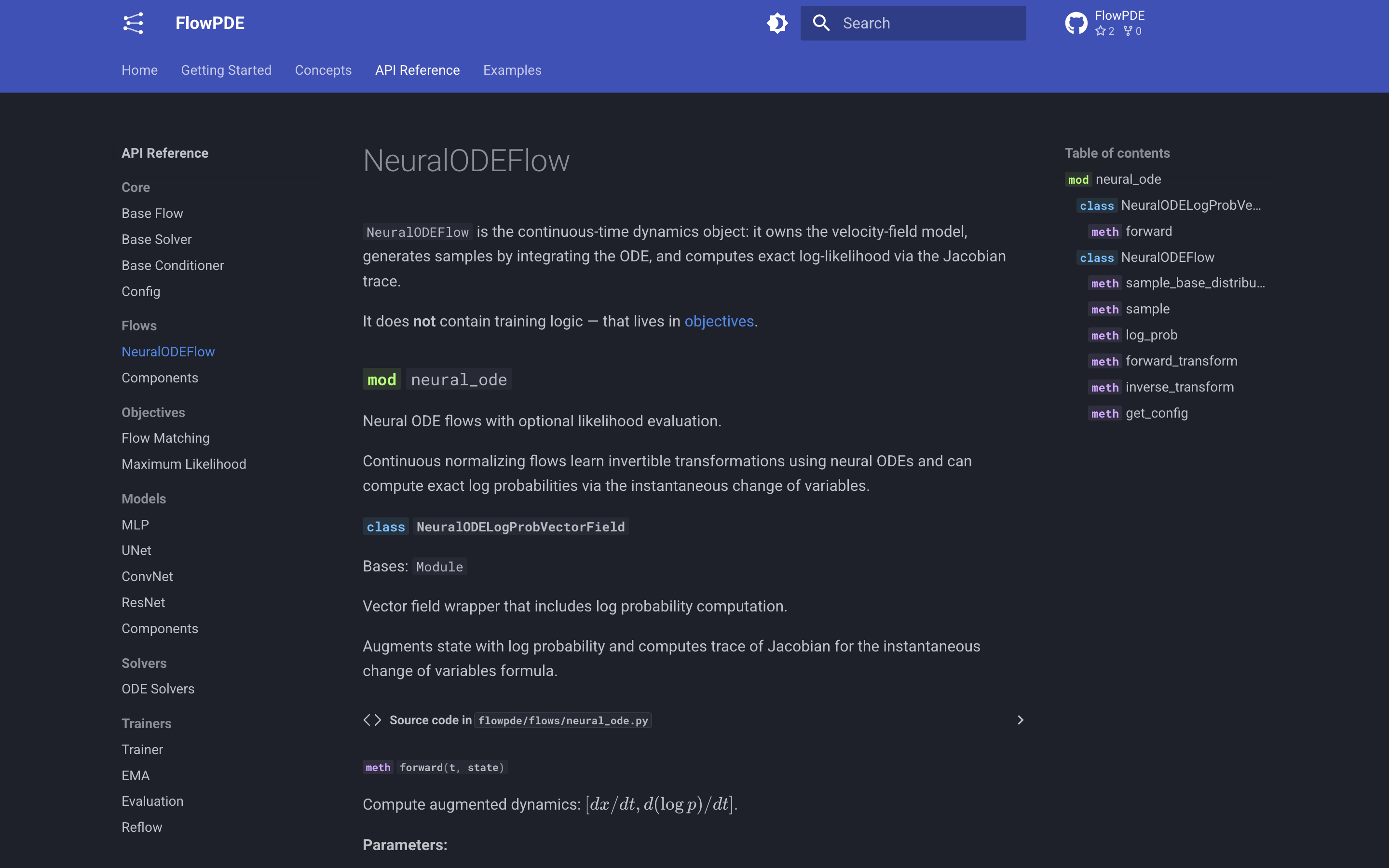
The documentation is hosted at sarperyn.github.io/FlowPDE.
It is built with MkDocs and API pages are generated from the docstrings by mkdocstrings, so they track the code rather than being written twice. Every push to main rebuilds and redeploys it through
.github/workflows/docs.yml.
Credits
No third-party code is included in this repository. Every module under flowpde/ was written specifically for this project, and the MIT licence applies to the entire codebase.
The library does, however, use methods from existing research. These include formulas, training schedules, and model architectures described in published papers and reimplemented here.
Methods implemented from the literature
| Component | Implements | Source |
|---|---|---|
flows/neural_ode.py |
Continuous normalizing flow; instantaneous change of variables | Chen et al., Neural Ordinary Differential Equations, NeurIPS 2018 · Grathwohl et al., FFJORD, ICLR 2019 |
flows/neural_ode.py |
Stochastic trace estimator | Hutchinson, A Stochastic Estimator of the Trace of the Influence Matrix, Commun. Stat. 1989 |
objectives/maximum_likelihood.py |
Maximum-likelihood training of a CNF | Rezende & Mohamed, Variational Inference with Normalizing Flows, ICML 2015 · Grathwohl et al., ICLR 2019 |
objectives/flow_matching.py, flows/components/paths.py |
Flow-matching objective; linear and OT-conditional paths | Lipman et al., Flow Matching for Generative Modeling, ICLR 2023 · Liu et al., Rectified Flow, ICLR 2023 · Tong et al., Improving and Generalizing Flow-Based Generative Models with Minibatch Optimal Transport, TMLR 2024 |
flows/components/couplings.py |
Mini-batch optimal-transport coupling | Tong et al., TMLR 2024 |
flows/components/time_samplers.py |
Logit-normal sampling of the flow time | Esser et al., Scaling Rectified Flow Transformers, ICML 2024 |
trainers/reflow.py, estimate_straightness |
Reflow; the straightness functional | Liu et al., ICLR 2023 |
trainers/ema.py |
Weight averaging, including the min(d, (1+n)/(10+n)) warmup schedule |
Ho et al., Denoising Diffusion Probabilistic Models, NeurIPS 2020, and its reference implementation |
models/components.py |
Sinusoidal time embedding | Vaswani et al., Attention Is All You Need, NeurIPS 2017 · Ho et al., NeurIPS 2020 |
models/unet.py |
Encoder–decoder with skip connections | Ronneberger et al., U-Net, MICCAI 2015 · Ho et al., NeurIPS 2020, for the time-conditioned variant |
models/resnet.py |
Residual basic block | He et al., Deep Residual Learning for Image Recognition, CVPR 2016 |
core/base_conditioner.py |
FiLM conditioning | Perez et al., FiLM: Visual Reasoning with a General Conditioning Layer, AAAI 2018 |
datasets/exponax/darcy.py |
Log-normal Gaussian-random-field coefficients; the Darcy benchmark setup | Li et al., Fourier Neural Operator for Parametric PDEs, ICLR 2021 |
utils/metrics.py |
Relative $L^2$ convention for operator learning | Kovachki et al., Neural Operator, JMLR 2023 |
utils/uq_metrics.py |
CRPS and the energy score | Gneiting & Raftery, Strictly Proper Scoring Rules, JASA 2007 · Székely & Rizzo, Energy Statistics, JSPI 2013 |
utils/uq_metrics.py |
Rank histogram; spread–skill ratio | Hamill, Interpretation of Rank Histograms, Mon. Weather Rev. 2001 · Fortin et al., Why Should Ensemble Spread Match the RMSE of the Ensemble Mean?, J. Hydrometeorol. 2014 |
A note on one deliberate reimplementation: utils/metrics.py
duplicates what neuraloperator's LpLoss already provides. That is on purpose and it
keeps the dependency footprint small.
Software
| Package | Used for | Cite |
|---|---|---|
| PyTorch | Models, training, autograd | Paszke et al., NeurIPS 2019 |
| torchdiffeq | ODE integration for sampling and likelihoods | Chen et al., NeurIPS 2018; dopri5 follows Dormand & Prince, JCAM 1980 |
| Exponax | Spectral PDE solvers and initial-condition generation | Koehler et al., APEBench, NeurIPS D&B 2024 |
| JAX | Backend for dataset generation | Bradbury et al., 2018 |
| SciPy | Linear assignment for the OT coupling | Virtanen et al., Nature Methods, 2020 |
The project report has full bibliographic entries for everything above and cites them in context.
1 maintainer

Metadata
1 maintainer
Release files for flowpde 0.1.0
For a detailed explanation of source distributions (sdists) and built distributions (wheels), please see the package formats documentation.
Source distribution (sdist)
| File | Size | Uploaded | |
|---|---|---|---|
| flowpde-0.1.0.tar.gz | 120.2 kB | Details |
Built distribution (wheel)
| File | Interpreter | ABI | Platform | Reset |
|---|---|---|---|---|
| flowpde-0.1.0-py3-none-any.whl | Python 3 | none | any | Details |
Total release size: 233.1 kB
Release files / flowpde-0.1.0.tar.gz
| Download URL | flowpde-0.1.0.tar.gz |
|---|---|
| Size | 120.2 kB |
| Tags | Source |
|
SHA-256 checksum How to use checksums |
8e32a3dfd8e261a7ff5a13d31614a8daebd7130eacdc99fed114b41d09fef68c
|
|
BLAKE2b-256 checksum How to use checksums |
4a4e123f4348033a5f4ce6dc717d0436e523d178e0cd9f3d313bda7eba6156cb
|
| Upload date | |
|
Uploaded using Trusted Publishing? What is trusted publishing? |
Yes |
| Uploaded via |
twine/7.0.0 CPython/3.13.14
|
Provenance
Provenance describes where a file came from. On PyPI, provenance is shared via attestations, which provide a verifiable record of the build or publishing details. View details, limitations and caveats.


PyPI Publish Attestation
PyPI verified that this artifact, at this checksum, originated from the publisher listed below.
Signed by GitHub Actions, verified by PyPI on Oct 6, 2026.
Transparency logRelease files / flowpde-0.1.0-py3-none-any.whl
| Download URL | flowpde-0.1.0-py3-none-any.whl |
|---|---|
| Size | 112.9 kB |
| Tags | Python 3 |
|
SHA-256 checksum How to use checksums |
7196588abf3fbe9e0db903f33678bfd0b18a308ce68bc38f521d41e5ad764c45
|
|
BLAKE2b-256 checksum How to use checksums |
3adb2a395b3a6cc1cfd896a453f97f11ed092b82daeeb05438b81a9353d097f9
|
| Upload date | |
|
Uploaded using Trusted Publishing? What is trusted publishing? |
Yes |
| Uploaded via |
twine/7.0.0 CPython/3.13.14
|
Provenance
Provenance describes where a file came from. On PyPI, provenance is shared via attestations, which provide a verifiable record of the build or publishing details. View details, limitations and caveats.
PyPI Publish Attestation
PyPI verified that this artifact, at this checksum, originated from the publisher listed below.
Signed by GitHub Actions, verified by PyPI on Oct 6, 2026.
Transparency log













