Frequency-domain model explanation (IG) package

Project description
freqIG
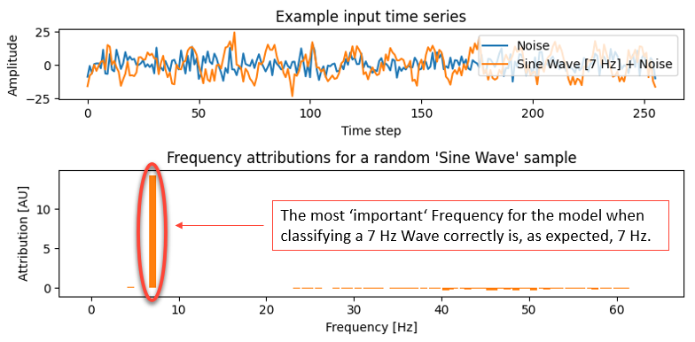
This is a basic example of this method, the code is given below in 'Examples'.
Overview
This repository contains the implementation of freqIG, a method based on the principle of FLEX (Frequency Layer Explanation) [1], designed to explain the predictions of deep neural networks (DNNs) for time-series classification tasks. freqIG combines Integrated Gradients (IG) with a frequency-domain transform (via the Real Fast Fourier Transform (RFFT)) to provide frequency-based attribution scores.
The method is generally useful for understanding how different frequency components of a time-series input influence the predictions of a DNN, thus enhancing model interpretability.
For details and an application of this method, see [1]: "Using EEG Frequency Attributions to Explain the Classifications of a Deep Neural Network for Sleep Staging" (Paul Gräve et al.). ~ soon to be published, if not already available
Features
- RFFT Transformation: Input time-series data are transformed into the frequency domain using the RFFT.
- iRFFT Transformation: The inverse RFFT (iRFFT) is implemented as the first layer in the DNN to process frequency-domain inputs.
- Integrated Gradients Attribution: Captum's IG method is used to compute relevance scores for frequency bands, providing insights into the features contributing to the model's predictions.
Definition (FLEX principle)
Let F be our model (DNN) and x be our input (time-series data). Then with
F̄ = F ∘ iRFFT and x̄ = RFFT(x) we get
$$ FLEXᵢ(F, x) = IGᵢ(F̄, x̄) $$
where
FLEX(F, x) = (FLEX₁(F, x), ..., FLEXₙ(F, x)) with x ∈ ℝⁿ.
Installation
Requirements
- Python 3.8+
- Required libraries:
numpytorchcaptum
- Optional libraries (for model conversion features):
onnxtf2onnxonnx2pytorch
Install the base package with required dependencies:
pip install freqig
To enable model conversion support (e.g., from ONNX or Keras), install with the optional extras:
pip install freqig[convert]
You can also install only specific optional dependencies if needed:
pip install freqig[onnx2pytorch]
pip install freqig[onnx]
pip install freqig[tf2onnx]
Documentation
freqIG.attribute
Compute frequency-based attribution scores for a model predicting on time-series data.
freqIG.attribute(
    input: Union[np.ndarray, list, torch.Tensor],
    model: Any,
    target: Optional[int] = None,
    baseline: Optional[Union[np.ndarray, list, torch.Tensor]] = None,
    n_steps: int = 50,
    segment: Optional[Union[np.ndarray, list, torch.Tensor]] = None,
    start_idx: Optional[int] = None,
    additional_forward_args: Optional[Any] = None
) -> np.ndarray
Parameters
-
input : array-like or torch.Tensor
The input time-series data. -
model : callable
The (frequency-domain) model to explain. -
target : int, optional
Index of the class to explain. If None, explains the model's predicted class. -
baseline : array-like or torch.Tensor, optional
Baseline input for Integrated Gradients. Defaults to zero input. -
n_steps : int, default=50
Number of steps in the IG path. -
segment : array-like or torch.Tensor, optional
Segment of the input for localized attribution. -
start_idx : int, optional
Start index of the segment within the original input. -
additional_forward_args : Any, optional
Additional arguments passed to the model during attribution.
Returns
- np.ndarray
Array containing the frequency attribution scores.
Raises
- ValueError
Ifsegmentis provided butstart_idxis missing, or if the segment exceeds the bounds of the input. - ValueError
Ifbaselineis provided but its shape does not match the input.
Notes
This function applies Integrated Gradients in the frequency domain to provide frequency-wise attributions for any model acting on time-series data, following the FLEX [1] principle.
References
[1] Using EEG Frequency Attributions to Explain the Classifications of a Deep Neural Network for Sleep Staging
Paul Gräve, T. Steinbrinker, F. Ehrlich, P. Hempel, P. Zaschke, D. Krefting, N. Spicher; 2025.
Examples
import sys
import os
sys.path.insert(0, os.path.abspath(os.path.join(os.path.dirname(__file__), '..')))
import numpy as np
from scripts.freqIG import attribute
import torch
import matplotlib.pyplot as plt

# Set seeds for reproducibility
np.random.seed(42)
torch.manual_seed(42)

# Define sampling rate in Hz and signal length:
fs = 128                # Sampling frequency, e.g. 128 Hz
n_samples = 100
n_features = 256         # Number of samples per time series

# Frequency axis in Hz:
freqs = np.fft.rfftfreq(n_features, d=1/fs)

# --- Select target frequency in Hz ---
possible_freqs_hz = np.arange(1, min(10, int(fs // 2)))  # Valid Hz, up to Nyquist
target_freq_hz = np.random.choice(possible_freqs_hz)
# Find closest matching index on the FFT axis:
target_freq_idx = np.argmin(np.abs(freqs - target_freq_hz))
target_freq = freqs[target_freq_idx]
print(f"Target frequency: {target_freq:.1f} Hz @ Index {target_freq_idx}")

# --- Generate data ---
X = []
y = []
t = np.arange(n_features) / fs  # Time axis in seconds

for i in range(n_samples):
    label = np.random.randint(0, 2)
    base = 5 * np.random.randn(n_features)
    if label == 1:
        phase = np.random.uniform(0, 2*np.pi)
        amplitude = np.random.uniform(10, 30)
        base += amplitude * np.sin(2 * np.pi * target_freq * t + phase)
    X.append(base)
    y.append(label)

X = np.stack(X)
y = np.array(y)

X_torch = torch.tensor(X, dtype=torch.float32)
y_torch = torch.tensor(y, dtype=torch.long)

class SimpleCNN(torch.nn.Module):
    def __init__(self):
        super().__init__()
        self.conv1 = torch.nn.Conv1d(1, 8, kernel_size=5, padding=2)
        self.relu1 = torch.nn.ReLU()
        self.conv2 = torch.nn.Conv1d(8, 16, kernel_size=3, padding=1)
        self.relu2 = torch.nn.ReLU()
        self.pool = torch.nn.AdaptiveAvgPool1d(1)
        self.fc = torch.nn.Linear(16, 2)
    def forward(self, x):
        if x.dim() == 2:
            x = x.unsqueeze(1)  # [batch, 1, time]
        x = self.conv1(x)
        x = self.relu1(x)
        x = self.conv2(x)
        x = self.relu2(x)
        x = self.pool(x)       # [batch, channels, 1]
        x = x.squeeze(-1)      # [batch, channels]
        return self.fc(x)

model = SimpleCNN()

# --- Training ---
criterion = torch.nn.CrossEntropyLoss()
optimizer = torch.optim.Adam(model.parameters(), lr=0.01)
model.train()
for epoch in range(150):
    optimizer.zero_grad()
    outputs = model(X_torch)
    loss = criterion(outputs, y_torch)
    loss.backward()
    optimizer.step()
model.eval()

# 1. Compute accuracy
with torch.no_grad():
    logits = model(X_torch)
    preds = torch.argmax(logits, dim=1).cpu().numpy()
    accuracy = np.mean(preds == y)
print(f"Model accuracy: {accuracy:.3f}")

# The first class 1 sample that is correctly classified by the model is used as an example
with torch.no_grad():
    logits = model(X_torch)
    preds = torch.argmax(logits, dim=1).cpu().numpy()

idx_candidates = np.flatnonzero((y == 1) & (preds == 1))
if len(idx_candidates) == 0:
    raise ValueError("No correctly classified class 1 samples found.")
idx = idx_candidates[0]
sample = X[idx:idx+1]

attr_scores = attribute(
    input=sample,
    model=model,
    target=1,        # Class 1 == "has the target frequency"
    n_steps=50
)

# --- Attribution visualization (as dictionary) ---
freq_axis = np.fft.rfftfreq(n_features, d=1)
attr_dict = {freq: score for freq, score in zip(freq_axis, attr_scores)}

# -----------------------------------------------------------------------------
# 2. Plot one example from class 0 and one from class 1
fig, axs = plt.subplots(2, 1, figsize=(8, 4), gridspec_kw={'height_ratios': [1, 1.8]})

ex0 = np.where(y == 0)[0][0]
ex1 = np.where(y == 1)[0][0]

# Plot 1 – Time series example
axs[0].plot(np.arange(n_features), X[ex0], label="Noise")
axs[0].plot(np.arange(n_features), X[ex1], label=f"Sine Wave [{target_freq_hz} Hz] + Noise")
axs[0].set_title("Example input time series")
axs[0].set_xlabel("Time step")
axs[0].set_ylabel("Amplitude")
axs[0].legend(loc='upper right')

# Plot 2 – Frequency attributions
bar_width = 0.8
axs[1].bar(freqs, attr_scores, width=bar_width, color='tab:orange')
axs[1].set_xlabel("Frequency [Hz]")
axs[1].set_ylabel("Attribution [AU]")
axs[1].set_title("Frequency attributions for a random 'Sine Wave' sample")

plt.tight_layout()
plt.savefig("freqIG_attributions.png")
print("Plots saved as: freqIG_attributions.png")
Release history Release notifications | RSS feed


Download files
Download the file for your platform. If you're not sure which to choose, learn more about installing packages.
Source Distribution
Built Distribution
Filter files by name, interpreter, ABI, and platform.
If you're not sure about the file name format, learn more about wheel file names.
Copy a direct link to the current filters
File details
Details for the file freqig-0.1.8.tar.gz.
File metadata
- Download URL: freqig-0.1.8.tar.gz
- Upload date:
- Size: 11.1 kB
- Tags: Source
- Uploaded using Trusted Publishing? No
- Uploaded via: twine/6.1.0 CPython/3.12.10
File hashes
| Algorithm | Hash digest | |
|---|---|---|
| SHA256 |
498e77bb3bf0b8f787bcd59b874d345217a6ff866e5b362a07be03b179e8dee7
|
|
| MD5 |
9747575f1eabe16ec86b7cda9466d44e
|
|
| BLAKE2b-256 |
84db866e595d814f99b3fdaf2f7414249e0bed82409b7d109c4c4fcdb69c15bc
|
File details
Details for the file freqig-0.1.8-py3-none-any.whl.
File metadata
- Download URL: freqig-0.1.8-py3-none-any.whl
- Upload date:
- Size: 8.8 kB
- Tags: Python 3
- Uploaded using Trusted Publishing? No
- Uploaded via: twine/6.1.0 CPython/3.12.10
File hashes
| Algorithm | Hash digest | |
|---|---|---|
| SHA256 |
f3d76167e190e84d63834fa11711adfa2f4508221cb2efc3b89705f877543760
|
|
| MD5 |
c3ad4fbbb3d007fcbec614c878c97a08
|
|
| BLAKE2b-256 |
61eb32212046ff11f52f28ee14a6a7074b8cb146becd8fb7b0314d8907a0ce24
|


