
FuncyFlows
Normalizing flows and flow matching on function spaces.
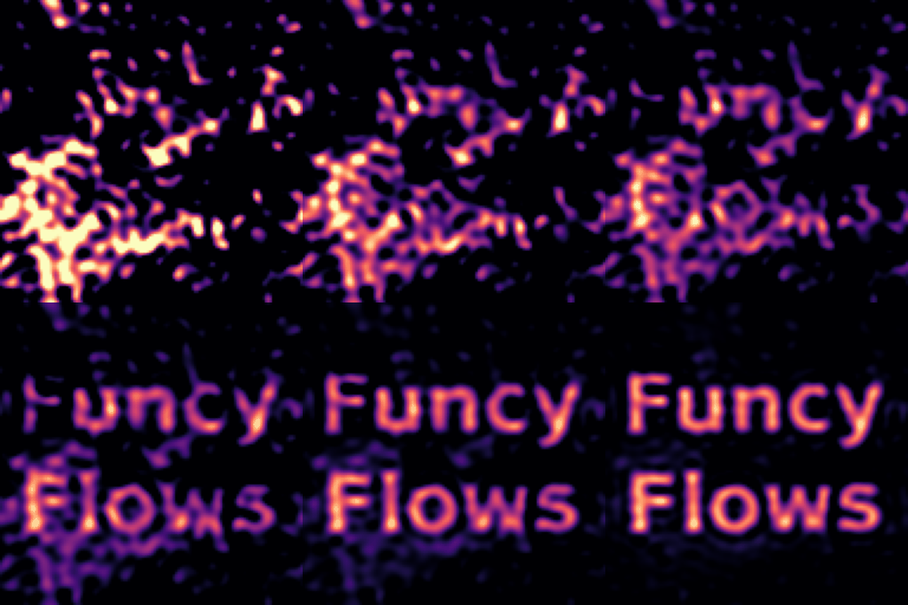
A function is represented by its coefficients on a Laplacian eigenbasis (CosineBasis or
FourierBasis), the reference measure is a Gaussian on those coefficients, and a transport is a
neural ODE in coefficient space. The vector fields (LinearField, MatrixField) have closed-form
divergences, so the density of the transported measure relative to the
reference measure is exact — no Hutchinson estimators — which makes reverse-KL training,
likelihood training and importance reweighting usable at hundreds of modes.
pip install funcyflows # torch + tqdm
Full documentation can be found here.
Examples
python -m FuncyFlows.examples        # copies the example scripts into the current directory
python bimodal_posterior.py         # then run any of them
| Script | What it shows |
|---|---|
bimodal_posterior.py |
1D, y = f² + noise: pCN vs Laplace-GP vs reverse KL vs flow matching vs exact latent pCN |
positivity.py |
1D log-normal prior: positivity and skew that no Gaussian reproduces |
nonstationary.py |
1D random-lengthscale prior: a mixture of GPs, scored by roughness spread |
ring_inpainting.py |
2D rings, central hole: learned prior + latent pCN vs GP with the same variances |
cloud_inpainting.py |
2D saturated power-law fields, 256 scattered points |
phase_inpainting.py |
2D two-phase fields: the posterior marginal is two spikes, a GP's is a smear |
The 2D examples and the two 1D prior examples use the spatial PointwiseField; the bimodal one is
coefficient-space only. Each takes 3–12 minutes on a CPU. Except for cloud inpainting and phase inpainting which can take up to 50mins.
The pieces
| Piece | Role |
|---|---|
CosineBasis(M), FourierBasis(M) |
M orthonormal basis functions on [0, 1]; basis.evaluate(points) → design matrix |
GaussianReferenceMeasure(basis, alpha, power) or (basis, variances=...) |
base measure N(0, diag σ²) on the coefficients; .sample(n), .scale (= σ) |
LinearField |
per-mode gain plus a data-dependent drift; exact for the linear-Gaussian part |
MatrixField(conditioner) |
one wide tanh layer over all coefficients; global nonlinear mixing |
SumField(*fields) |
add fields; traces add |
ContinuousTransformation(measure, field, num_steps) |
the flow: .transport(v0), .push_forward, .pull_back, .log_rn_at(v) |
FlowMatching, ConditionalFlowMatching, ReverseKL, NegativeLogL |
objectives; each is a callable returning a loss |
train(objective, params, num_steps, learning_rate) |
Adam loop, returns the loss history |
ImportanceCorrection, coverage_curve, latent_pcn |
diagnostics and an exact latent-space MCMC sampler |
Every field takes mode_scale=measure.scale: the nonlinearity sees whitened coefficients and the
divergence is unchanged (similarity transform). Always pass it.
1. Learn a prior from samples (flow matching)
import torch
from FuncyFlows.base_measures import CosineBasis, GaussianReferenceMeasure
from FuncyFlows.transports.continuous import (ContinuousTransformation, SumField, LinearField,
                                             MatrixField, TimeBasisConditioner)
from FuncyFlows.objectives import FlowMatching
from FuncyFlows.utils.train import train

M = 64
basis = CosineBasis(M)
coeffs = ...                                  # [N, M] training functions projected onto the basis
measure = GaussianReferenceMeasure(basis, variances=coeffs.var(0))   # diagonal Gaussian fit = the GP baseline

field = SumField(
    LinearField(M, num_time_modes=4),
    MatrixField(TimeBasisConditioner(M, 256, num_time_modes=4), mode_scale=measure.scale))
flow = ContinuousTransformation(measure, field, num_steps=16)

losses = train(FlowMatching(flow, coeffs, batch_size=256, weights=1 / measure.scale, coupling="optimal"),
               flow.parameters(), num_steps=10000, learning_rate=2e-3)

draws = flow.transport(measure.sample(1000))              # [1000, M] new functions
points = torch.linspace(0, 1, 400).reshape(-1, 1)
values = draws @ basis.evaluate(points).T                 # [1000, 400] on a grid
log_q = flow.log_rn_at(draws)                             # exact log density w.r.t. the reference measure
weights=1/measure.scale whitens the loss so high modes count; coupling="optimal" needs
scipy and only makes sense for an unconditional flow.
2. Posterior from a likelihood (no samples needed)
from FuncyFlows.objectives import ReverseKL
from FuncyFlows.utils.gaussian_misfit import GaussianMisfit
from FuncyFlows.diagnostics import ImportanceCorrection

prior = GaussianReferenceMeasure(basis, alpha=0.05, power=2.0)     # Matérn-like spectrum
phi_obs = basis.evaluate(obs_points)                               # [n_obs, M]
forward = lambda v: (v @ phi_obs.T) ** 2                           # any differentiable map
potential = GaussianMisfit(forward, data, noise_std)               # -log likelihood, [batch] -> [batch]

flow = ContinuousTransformation(prior, field, num_steps=16)        # same field recipe as above
train(ReverseKL(flow, potential, num_samples=64, path_gradient=True), flow.parameters(), num_steps=3000)

draws = flow.transport(prior.sample(2000))
check = ImportanceCorrection(flow, draws, potential)               # exact because the traces are exact
print(check.efficiency, check.log_evidence)                        # efficiency near 1 = posterior matched
For an exact sampler on top of a learned prior use latent_pcn(flow, potential): pCN in the flow's
latent space, whose acceptance needs no Jacobian.
3. Amortised posterior (condition on data)
from FuncyFlows.transports.continuous import DataConditioner
from FuncyFlows.objectives import ConditionalFlowMatching

C = ...                                                    # context dimension (e.g. whitened projected data)
field = SumField(
    LinearField(M, C, num_time_modes=4, mode_scale=measure.scale),          # data drift: the linear-Gaussian mean
    MatrixField(DataConditioner(M, 256, C, num_time_modes=4), mode_scale=measure.scale))
flow = ContinuousTransformation(measure, field, num_steps=16)

def simulate(batch):                                       # -> (target coeffs [batch, M], context [batch, C])
    ...

train(ConditionalFlowMatching(flow, simulate, measure.sample, batch_size=256, weights=1 / measure.scale),
      flow.parameters(), num_steps=20000, learning_rate=2e-3)

posterior = flow.transport(measure.sample(1000), context.expand(1000, -1))   # one ODE solve per posterior
Whiten the context by measure.scale when it is itself a projected function; otherwise the drift
weights for high modes have to reach 1/σ and never do. When a conjugate (linear-Gaussian)
posterior is available in closed form, use it as the base measure and let the flow learn the residual.
Diagnostics
from FuncyFlows.diagnostics import coverage_curve, coverage_error
levels, coverage = coverage_curve(samples, truths, weights=1 / measure.scale)   # TARP; samples [cases, draws, M]
coverage_error(levels, coverage)     # signed max gap from the diagonal: negative = overconfident
Layout
FuncyFlows/
  base_measures/     bases, GaussianReferenceMeasure
  transports/        continuous/: fields, conditioners, ContinuousTransformation
                     (grid_fields.py: PointwiseField, one FNO-style spatial layer with exact trace)
  examples/          python -m FuncyFlows.examples
  objectives/        flow_matching, reverse_kl, negative_logl
  samplers/          latent_pcn
  diagnostics/       importance, coverage
  utils/             train, gaussian_misfit
1 maintainer

Metadata
1 maintainer
Release files for funcyflows 0.2.2
For a detailed explanation of source distributions (sdists) and built distributions (wheels), please see the package formats documentation.
Source distribution (sdist)
| File | Size | Uploaded | |
|---|---|---|---|
| funcyflows-0.2.2.tar.gz | 60.6 kB | Details |
Built distribution (wheel)
| File | Interpreter | ABI | Platform | Reset |
|---|---|---|---|---|
| funcyflows-0.2.2-py3-none-any.whl | Python 3 | none | any | Details |
Total release size: 136.2 kB
Release files / funcyflows-0.2.2.tar.gz
| Download URL | funcyflows-0.2.2.tar.gz |
|---|---|
| Size | 60.6 kB |
| Tags | Source |
|
SHA-256 checksum How to use checksums |
77233e5f072572aa593a9ee06a33aec5e3007e2802cb6afd6b9d1a68f44821e6
|
|
BLAKE2b-256 checksum How to use checksums |
3e640b82318760fe6a4cd1676a92fab17e66aeda2f77e4ac7d0262b1f84f7e1f
|
| Upload date | |
|
Uploaded using Trusted Publishing? What is trusted publishing? |
No |
| Uploaded via |
twine/7.0.0 CPython/3.13.5
|
Release files / funcyflows-0.2.2-py3-none-any.whl
| Download URL | funcyflows-0.2.2-py3-none-any.whl |
|---|---|
| Size | 75.6 kB |
| Tags | Python 3 |
|
SHA-256 checksum How to use checksums |
5935b8da8aba6dd4577000f09c1644a6ec8b80117a471333bd8c745976632d06
|
|
BLAKE2b-256 checksum How to use checksums |
5bde14dd4c6361782d60c788ce3ce7684a321b4468075308c8d75091c071f028
|
| Upload date | |
|
Uploaded using Trusted Publishing? What is trusted publishing? |
No |
| Uploaded via |
twine/7.0.0 CPython/3.13.5
|














