
Gaste Package
Welcome to the Gaste package! This package provides a set of tools and utilities for analyzing stratified 2x2 contingency table. Gives the exact or approximate p-value of the overall association between features and outcomes under 2x2 stratified contingency table.
Citation
If you use the package GASTE in your project, please cite us :
Installation
To install the Gaste package, simply run the following command:
pip install gaste-test
Basic import
Once installed, you can import the Gaste package or the main function in your Python code using the following line:
import gaste-test
from gaste-test import get_pval_comb, StratifiedTable2x2
Features
The Gaste package offers the following features:
- Exact calcul of p-value combination of one tail Fisher's exact test
- Approximation of the law of combination by Gamma approximation distribution
- Incorporating truncation into the p-value combination enhances statistical power in scenarios featuring few effects or contradictory effects between strata
- Visualization: Forest plot for data analysis.
Example of use
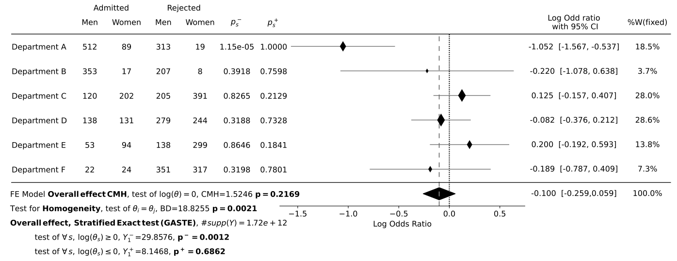
Example of Berkeley's admission in 1973 by departement and gender :
>>> admission = pd.read_csv("admission.csv")
| Department | Male-Admitted | Female-Admitted | Male-Rejected | Female-Rejected |
|---|---|---|---|---|
| A | 512 | 89 | 313 | 19 |
| B | 353 | 17 | 207 | 8 |
| C | 120 | 202 | 205 | 391 |
| D | 138 | 131 | 279 | 244 |
| E | 53 | 94 | 138 | 299 |
| F | 22 | 24 | 351 | 317 |
    # Data preparation
>>> nb_strata = admission.shape[0]
>>> rows = ("Admitted", "Rejected")
>>> columns = ("Men", "Women")
>>> contingency_table = np.array(
        admission.loc[:, admission.columns != "Department"]
    ).reshape((nb_strata, 2, 2))
>>> strat_label = ["Department " + dep for dep in admission["Department"]]
    # Create object
>>> stratified_table = StratifiedTable2x2(
        contingency_table, labels=strat_label, name_rows=rows, name_columns=columns
    )
>>> stratified_table.resume()
| Studies | Men Admitted | Women Admitted | Men Rejected | Women Rejected | $p_s^-$ | $p_s^+$ | OR | log(OR) | CI | log(CI) | %W(fixed) |
|---|---|---|---|---|---|---|---|---|---|---|---|
| Department A | 512 | 89 | 313 | 19 | 1.15063e-05 | 0.999996 | 0.349 | -1.052 | [0.209, 0.584] | [-1.567, -0.537] | 18.5 |
| Department B | 353 | 17 | 207 | 8 | 0.391761 | 0.759839 | 0.803 | -0.22 | [0.340, 1.892] | [-1.078, 0.638] | 3.7 |
| Department C | 120 | 202 | 205 | 391 | 0.826548 | 0.212876 | 1.133 | 0.125 | [0.855, 1.502] | [-0.157, 0.407] | 28 |
| Department D | 138 | 131 | 279 | 244 | 0.318816 | 0.73277 | 0.921 | -0.082 | [0.686, 1.237] | [-0.376, 0.212] | 28.6 |
| Department E | 53 | 94 | 138 | 299 | 0.864569 | 0.184058 | 1.222 | 0.2 | [0.825, 1.809] | [-0.192, 0.593] | 13.8 |
| Department F | 22 | 24 | 351 | 317 | 0.319845 | 0.780128 | 0.828 | -0.189 | [0.455, 1.506] | [-0.787, 0.409] | 7.3 |
Pooled odd ratio with MH method : 0.9047
Confident interval at 95.0% of pooled odd ratio : (0.7719, 1.0603)
>>> stratified_table.nb_combination
1719197241840
>>> stratified_table.gaste(alternative='less')
The support of the combined p-value is 1.72e+12, over the compute explicite threshold of 1.00e+07 , the moment matching estimator is used.
statistic: 29.8576, p-value: 0.0012
>>> stratified_table.gaste(alternative='greater')
The support of the combined p-value is 1.72e+12, over the compute explicite threshold of 1.00e+07 , the moment matching estimator is used.
statistic: 8.1468, p-value: 0.6862
>>> stratified_table.plot(thresh_adjust=0.03, save="analysis_admission.png")
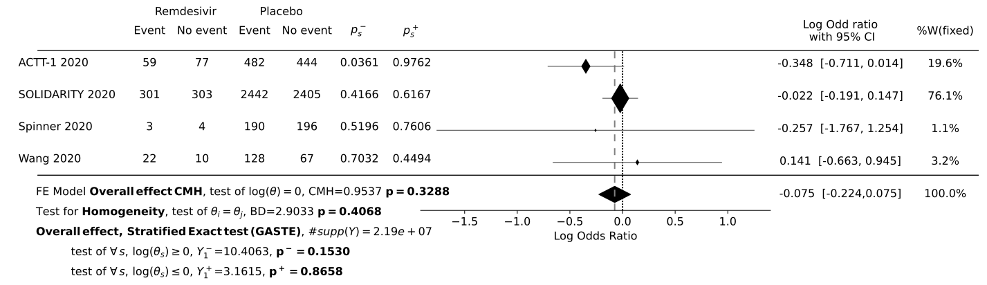
Example: Razzack AA, Hassan SA, Pasya SKR, et al. A Meta-Analysis of Association between Remdesivir and Mortality among Critically-Ill COVID-19 Patients. Infect Chemother. 2021;53(3):512-518. doi:10.3947/ic.2021.0060
>>> contingency_table = [
        [[59, 77], [482, 444]],
        [[301, 303], [2442, 2405]],
        [[3, 4], [190, 196]],
        [[22, 10], [128, 67]],
    ]
>>> strat_label = ["ACTT-1 2020", "SOLIDARITY 2020", "Spinner 2020", "Wang 2020"]
>>> rows = ("Remdesivir", "Placebo")
>>> columns = ("Event", "No event")
>>> stratified_table = StratifiedTable2x2(
        contingency_table, labels=strat_label, name_rows=rows, name_columns=columns
    )
>>> stratified_table.nb_combination
21881640
>>> stratified_table.gaste(alternative='less')
The support of the combined p-value is 2.19e+07, over the compute explicite threshold of 1.00e+07 , the moment matching estimator is used.
statistic: 29.8576, p-value: 0.1527
>>> stratified_table.gaste(alternative='greater')
The support of the combined p-value is 2.19e+07, over the compute explicite threshold of 1.00e+07 , the moment matching estimator is used.
statistic: 8.1468, p-value: 0.8658
    # Force exact calculation by increasing the limit threshold of exact computation
>>> stratified_table.gaste(alternative='less', limit_computation_exact=3*10**7)
The support of the combined p-value is 2.19e+07, under the compute explicite threshold of 3.00e+07 , the explicite calculation is used.
[137, 605, 8, 33] size 21881640
100%|██████████████████████████████████████████████████████| 21881640/21881640 [00:41<00:00, 524130.92it/s]
statistic: 29.8576, p-value: 0.1529
>>> stratified_table.plot(thresh_adjust=0.03, save="analysis_admission.png")
Example without object StratifiedTable2x2, only get_pval_comb function
    # Data from Rothman, K.J. (1982). "Spermicide use and Down's syndrome," American Journal of Public Health, 72(4), pp. 399-401. doi 10.2105/AJPH.72.4.399.
>>> contingency_table = [[[3, 9], [104, 1059]], [[1, 3], [5, 89]]]
    # Format data to get (sample size, marginal A, marginal B)
>>> params = np.vstack((np.sum(contingency_table, axis=(1,2)), np.sum(contingency_table, axis=2).T[0], np.sum(contingency_table, axis=1).T[0])).T
>>> params
array([[1175,   12,  107],
       [  98,    4,    6]])
>>> # Same as : params = [[3+9+104+1059, 3+9, 3+104], [1+3+5+89, 1+3, 1+5]]
    # computation of p-value
>>> from scipy.stats import hypergeom
>>> pval_under = [hypergeom(*param).cdf(k) for param, k in zip(params, np.array(contingency_table)[:,0,0])]
>>> pval_under
[0.9818678457734665, 0.9821041004573289]
>>> pval_over = [hypergeom(*param).sf(k-1) for param, k in zip(params, np.array(contingency_table)[:,0,0])]
>>> pval_over
[0.08808167695347509, 0.2264843810557321]
>>> from gaste_test import get_pval_comb
>>> get_pval_comb(params, pval_under, "under")
0.9946415406410173
>>> get_pval_comb(params, pval_over, "over")
0.05029422728685044
Example of R wrapper with reticulate
As input to the StratifiedTable2x2 object, we have presented a contingency table in the form of an array of shape (nb_strat, 2,2) as. But we can also give as input a list of tuples 4 integers representing ($N_s$, $n_s$, $K_s$, $a_s$) where $N_s$ is the total count of events and non-events, $n_s$ is the count of events in both categories, $K_s$ is the total count in the first category, and $a_s$ is the count of events in the first category. This is illustrated below when using the package in R through reticulate
> library(reticulate)
> py_install("gaste-test")
> gaste <- import("gaste_test", delay_load = TRUE, convert = TRUE)
> params <- list(c(300, 80, 60, 15),
+                c(300, 70, 50, 5),
+                c(250, 130, 40, 20),
+                c(300, 80, 60, 18))
> params_ <- r_to_py(params)
> stb <- gaste$StratifiedTable2x2(params_)
> stb$resume()
           $k_s$  $K_s-k_s$  ...           log(CI)  %W(fixed)
Studies                      ...
Stratum 0     15         45  ...   [-0.758, 0.542]       26.4
Stratum 1      5         45  ...  [-2.117, -0.185]       26.4
Stratum 2     20         20  ...   [-0.772, 0.581]       23.8
Stratum 3     18         42  ...   [-0.416, 0.831]       23.5

[4 rows x 11 columns]

Pooled odd ratio with MH method :  0.8251
Confident interval at 95.0% of pooled odd ratio : (0.586, 1.1618)
> stb$gaste('less')
The support of the combined p-value is 7.78e+06, under the compute explicite threshold of 1.00e+07 , the explicite calculation is used.
[61, 51, 41, 61] size 7780611 max supp 61
100%|██████████| 7780611/7780611 [00:12<00:00, 640481.60it/s]
statistic: 13.1942, p-value: 0.0586
> stb$gaste('greater')
The support of the combined p-value is 7.78e+06, under the compute explicite threshold of 1.00e+07 , the explicite calculation is used.
[61, 51, 41, 61] size 7780611 max supp 61
100%|██████████| 7780611/7780611 [00:12<00:00, 621091.29it/s]
statistic: 3.9103, p-value: 0.7847
> stb$plot(save='test.png')
Documentation
For detailed information on how to use the Gaste package, please refer to the sphinx documentation : https://gaste.readthedocs.io/en/latest/
Contributing
We welcome contributions from the community! If you would like to contribute to the Gaste package, feel free to contact the autor by mail.
License
The Gaste package is licensed under the MIT License.
1 maintainer

Release files for gaste-test 0.1.6
For a detailed explanation of source distributions (sdists) and built distributions (wheels), please see the package formats documentation.
Built distribution (wheel)
| File | Interpreter | ABI | Platform | Reset |
|---|---|---|---|---|
| gaste_test-0.1.6-py3-none-any.whl | Python 3 | none | any | Details |
Release files / gaste_test-0.1.6-py3-none-any.whl
| Download URL | gaste_test-0.1.6-py3-none-any.whl |
|---|---|
| Size | 20.5 kB |
| Tags | Python 3 |
|
SHA-256 checksum How to use checksums |
f9042f25c5029f4abf48593517a8e79f16b951a72ba1d880b003326d67afce27
|
|
BLAKE2b-256 checksum How to use checksums |
dd73e9df06252516d813853c3b76a85877b2cd4de2333acea268493ced33c342
|
| Upload date | |
|
Uploaded using Trusted Publishing? What is trusted publishing? |
No |
| Uploaded via |
twine/5.1.1 CPython/3.10.12
|














