
gathervis
English | 简体中文
A professional web viewer for pre-stack seismic data.
Open pre-stack data sitting on a remote server in your browser, and work it the way you would in processing software: browse shots, filter, take spectra, pick.



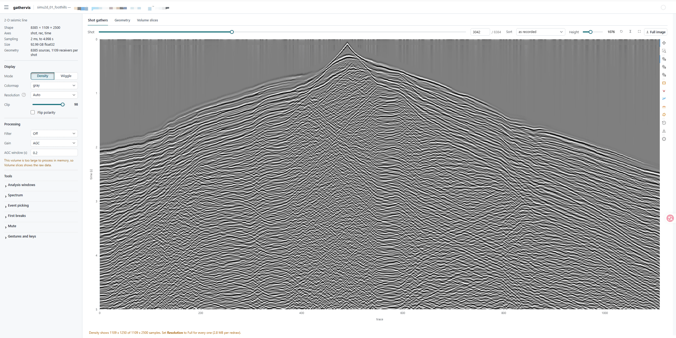
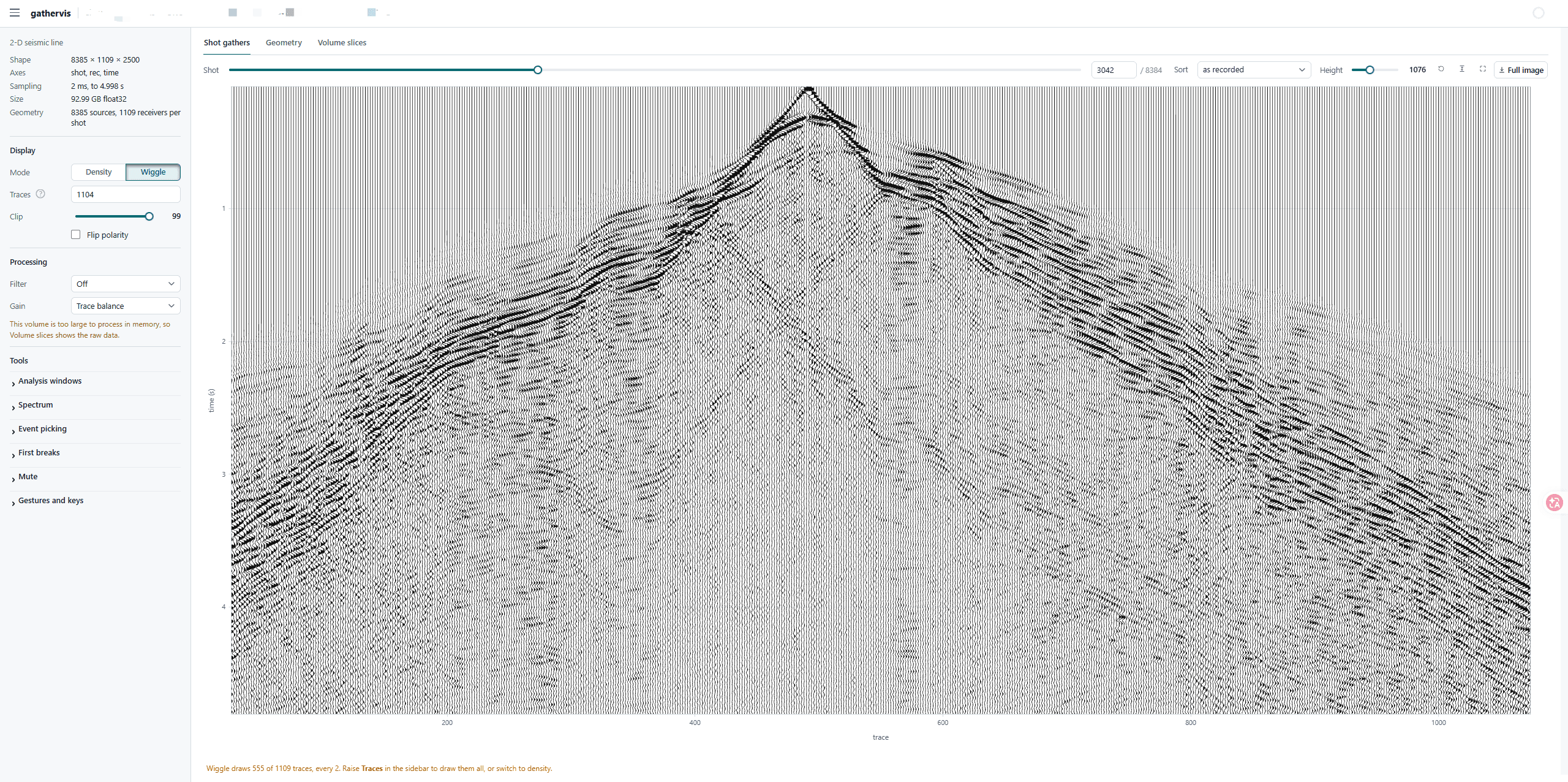
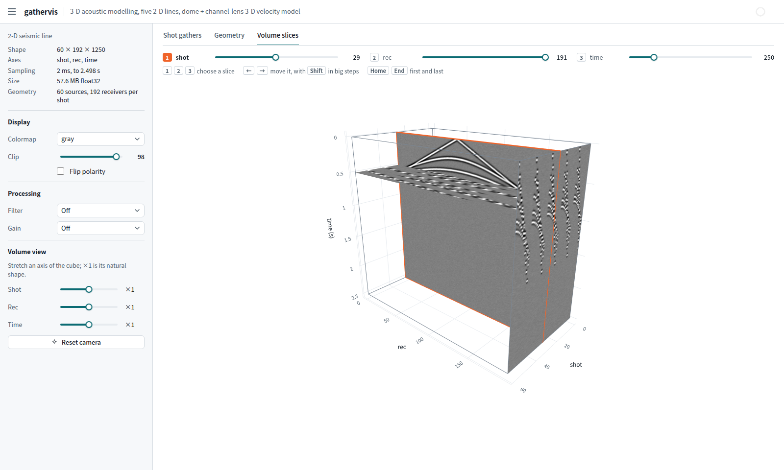
2-D gather QC and 3-D volume slicing, in one browser tab.
💬 Feature requests welcome! If there is anything you wish it did — a display mode, a processing step, a file format — please open an issue and tell me. I will implement it. Thank you very much!
💬 欢迎提需求! 如果你希望它能做什么 —— 显示方式、处理步骤、文件格式 —— 请务必开 issue 告诉我,我会实现的,非常感谢!
Why gathervis?
The reason is a practical one: not wanting to draw pre-stack data with matplotlib one figure at a time. Change shot, redraw. Change a filter parameter, redraw. Want the spectrum of one time gate and that is another block of code. The figures come out fine, but the process is broken up, and every look starts over. gathervis turns it into the kind of viewing you get in processing software: the data is simply open in a browser, a slider steps through shots, drawing a box gives you its spectrum, and changing the filter updates the panel as you type.
- Instant on huge data. Files open as lazy memmaps — browsing a shot reads only that shot's bytes; slicing a volume reads only that slice. A 100 GB raw binary opens as fast as a 1 MB one.
- Geometry-linked views. Give it source/receiver coordinates and you get a Geometry tab with the CMP fold under the layout — tap any source point to jump to its shot gather, with the active spread highlighted; CMP fold is computed from coordinates alone.
- QC tools built in. Wiggle & variable-density display with industry colormaps, zero-phase Ormsby filters, AGC / trace balance, draw-a-window spectral analysis (amplitude spectra and f-k), manual / STA-LTA first-break picking, top / bottom mutes that carry across gathers, and hand-picked CMP velocity analysis.
- cigvis-style 3-D. Volumes render as a rotatable cuboid with three live slice planes (WebGL), moved by slider or keyboard.
- A quiet interface. The sidebar is grouped into display, processing and tools, and shows only the controls that act on what is on screen. Shots, slices and gathers step from the keyboard. The page fetches nothing from the internet, so it loads the same on an offline cluster or behind a firewall.
- Simple. All it needs is a browser: one port, auto-forwarded by VS Code
Remote-SSH, rendered inline in Jupyter, and reachable over a bare
ssh -L. Four dependencies, installed with pip.
Install
pip install -e .                  # numpy + panel + bokeh + plotly
pip install -e ".[segy]"          # optional, for SEG-Y import
pip install -e ".[examples]"      # optional, torch + deepwave for the
                                  # modelling examples -- ~2.5 GB
With uv, the extras are the same names:
uv sync                           # the viewer
uv sync --extra examples          # + torch/deepwave for examples/deepwave_*.py
uv run --extra examples examples/deepwave_line2d.py    # or just for one run
pyproject.toml pins torch to the cu121 wheel index for local development.
Without a GPU, or to keep the download small, point uv at the CPU index:
--index https://download.pytorch.org/whl/cpu. Only the two deepwave_*
examples need any of this; everything else runs on the four base
dependencies.
Quick start
import gathervis as gv

# -- quick look, no geometry --
gv.show(gather_2d, dt=0.002, port=8080)          # a (trace, time) panel
gv.show(line_3d, dt=0.002, port=8080)            # default (shot, rec, time): browse shots
gv.show(line_3d, view='slices', port=8080)       # same array as a 3-D cuboid w/ slices
gv.show('shots.bin', shape=(60,192,1200),        # raw binary: lazy memmap, opens instantly
        dtype='float32', dt=0.002, port=8080)
gv.show(vel, axes=('x','y','depth'), dt=10.0)    # property volume (velocity QC)

# -- with acquisition geometry --
ds = gv.from_array(data, src=src_xyz, rec=rec_xyz, dt=0.002)
gv.show(ds, port=8080)   # + Geometry tab; tap a source -> its shot gather
Or from the shell, no code at all:
gathervis line2d_data.npy --geom line2d_geom.npz
gathervis shots.bin --shape 60 192 1200 --dt 0.002
gathervis field.sgy                                # SEG-Y: dt + geometry from headers
gathervis vel.npy --axes x y depth --dt 10 --cmap rainbow
Examples with synthetic data: python examples/quickstart.py serves an
analytic synthetic; python examples/velocity_picking.py opens velocity
analysis on a CMP gather whose answer is known;
python examples/deepwave_line2d.py models a 2-D line with
deepwave; and
python examples/deepwave_lines3d.py shoots five 2-D lines over a rich 3-D
velocity model (dipping layers + anticline dome + low-velocity channel lens)
with deepwave's 3-D engine, then opens the result.
Features
Shot browsing and geometry
On the Shot gathers tab, the toolbar above the panel holds the shot slider (it updates the panel while you drag), a box to type a shot number into and, for 3-D shots, the sort; ← / → step one shot at a time, Shift makes it ten, Home / End go to the first and last shot. The view controls sit at the right of the same row, so they stay within reach in fullscreen.
The sidebar is grouped the way a look at the data goes: Display (density or wiggle, then only what that mode uses: colormap and resolution for density, trace count for wiggle; clip; polarity), Processing (filter and gain, each showing its parameters only when it is on), and Tools: Analysis windows, Spectrum, Event picking, First breaks and Mute as collapsible sections, with the gesture sheet as the last one. Tabs that have settings of their own add a section while they are showing: the Geometry tab its map layers and CMP bins, the volume tabs their axis stretch.
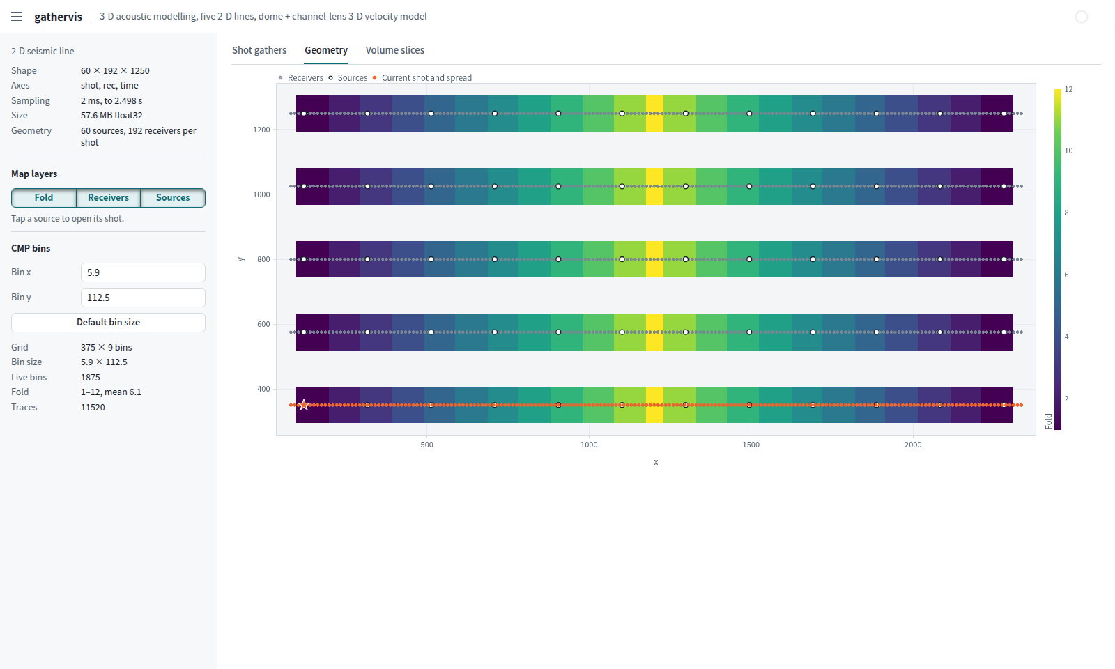
The Geometry tab is one map: the CMP fold underneath, sources and receivers on top, the current shot starred and its spread highlighted. Tapping a source selects that shot and returns to the Shot gathers tab; Map layers in the sidebar switches fold, receivers and sources on and off.
Trace ordering for 3-D shots
A 3-D shot is a patch of several receiver lines. Processing practice puts the
whole patch on one (trace, time) panel and changes the order the traces are
laid out in; the Sort selector on the Shot gathers tab provides four
orderings.

The same shot in three orderings: as recorded (receiver-line breaks dashed), by offset, by azimuth.
| sort | description |
|---|---|
as recorded (line, station) |
Acquisition order, receiver lines end to end, displayed as N nested hyperbolas whose apices step with cross-line distance. Used to check geometry errors, reversed lines, polarity flips and dead channels. Dashed separators mark the line boundaries. |
| receiver line | One receiver line at a time, i.e. a 2-D shot record. |
| offset | Ordered by source-receiver distance; the patch collapses onto one hyperbola. Used for moveout, mute design and velocity analysis. |
| azimuth | Ordered by source-to-receiver azimuth (survey convention, north = 0). Used for azimuthal behaviour and azimuth coverage. |
All four orderings are the same 2-D panel, so analysis windows, spectra, picking and full-resolution export work identically on them. Picks are stored against the trace rather than the screen column, so they follow a re-sort; picks on traces outside a single-line view are hidden rather than deleted and return when the view does.
offset and azimuth require geometry; receiver line requires 4-D
(shot, recy, recx, time) data, the shape in which the line structure is
explicit. The selector lists only the orderings the dataset supports, and is
hidden for a 2-D line with no geometry. The Shot volume tab renders the
current shot as a cuboid on the same filter/gain chain.
Example: python examples/quickstart.py patch.
CMP fold map
Underneath the acquisition layout on the Geometry tab — the same survey asked two ways, so a hole in the fold is a gap in the layout right on top of it. The fold bins the midpoint of every source-receiver pair on a rectangular grid, centred on the first midpoint so that regular midpoints fall mid-bin, and counts them. CMP bins in the sidebar sets the bin size and lists the grid, the live bins, the fold range and the trace count.
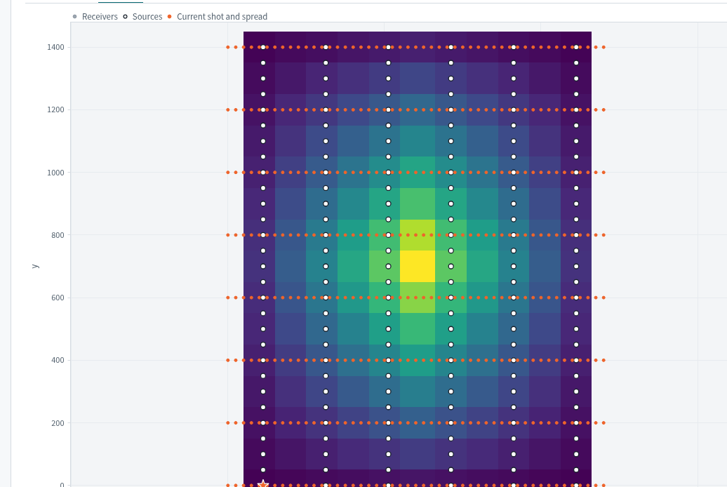
Fold of an orthogonal land 3-D: 25 m stations on 200 m receiver lines, 50 m shot points on 200 m shot lines half a station off the receiver stations, fixed full spread.
Bin size defaults to half the receiver station interval in-line and half the
line interval cross-line, the natural CMP sampling; both are editable under
CMP bins in the sidebar, and Default bin size restores them. Fold is drawn
in viridis, and empty bins in the background colour rather than at the bottom
of the colour scale. The list under the bin size gives the grid, the live
bins, the fold range and mean, and the trace total — which should equal
sources × receivers and serves as a geometry check.
The computation uses coordinates only and reads no trace data, so its cost is
independent of data volume and it works on a bare Geometry:
from gathervis.survey import fold, default_bin
grid = fold(ds.geometry)                     # or fold(geo, (12.5, 100.0))
grid.counts                                  # (ny, nx) traces per bin
grid.nlive, grid.extent, grid.bin_of(x, y)
Tapping a bin selects and outlines it. The trace index behind it — which
shot and which channel images the bin — is traces_in_bin; the offset-azimuth distribution comes
from the same module, though the in-app rose diagram is not yet implemented:
from gathervis.survey import (traces_in_bin, offsets_azimuths_in_bin,
                              azimuth_sectors)
shots, recs, offs = traces_in_bin(ds.geometry, grid, ix, iy)   # offset-sorted
offs, azis, shots = offsets_azimuths_in_bin(ds.geometry, grid, ix, iy)
edges, counts = azimuth_sectors(azis, nsector=24)   # survey convention, N = 0
The number of non-empty sectors returned by azimuth_sectors is the bin's
azimuth coverage.
Top and bottom mutes
Two point tools on the gather panel, one per line: tap to add a node, drag to move it, BACKSPACE deletes the selected one. The cut is drawn across every trace, so what you see is what will be applied rather than the handles you placed. Turn on Apply mute to see the gather with it — you cannot tell whether a cut is in the right place without seeing what it removes.
The lines are stored against offset, not against the column you dropped the node on. A mute is an offset-dependent thing, so a line stored that way means the same cut on the next shot even though that shot has different traces in a different order, and it survives re-sorting the panel. Without geometry there are no offsets and the line falls back to trace index, which is honest but does not travel between gathers.
One line serves everything, with exceptions. Edits go to decides where an edit goes — All gathers writes the default that every gather inherits, This gather gives the current one a line of its own. Make default pushes a line you tuned on one gather out to the rest; Revert drops an exception. The status line at the foot of the Mute section always says which of the two you are looking at. Nothing is interpolated between gathers: a gather either has its own line or uses the default.
Export writes JSON, and the same file mutes a gather from a script with no viewer involved:
from gathervis.mute import Mutes, mute_shot

mutes = Mutes.from_json(open("mutes.json").read())
clean = mute_shot(ds, 7, mutes)        # shot 7's own line if it has one
The pieces underneath work on any gather and its offsets:
from gathervis import mute

top = mute.linear_line(v=1500., x_max=3000., pad=0.05)   # a straight cut
out = mute.apply(gather, offsets, dt, top=top, taper=0.04)
mute.evaluate(top, offsets)                              # the cut time per trace
The taper is not decoration. A hard cut leaves a step running along the mute trajectory, and a step is broadband energy on a coherent path — it comes back in spectra and stacks as an event that was never in the ground.
Velocity analysis
from gathervis import cmp, survey
import gathervis as gv

grid = survey.fold(ds.geometry)
cg = cmp.gather_in_bin(ds, grid, ix, iy)
gv.velocity_analysis(cg, dt=ds.dt, port=8080)
Three panels reading left to right, which is the order the work happens in: the CMP gather, its semblance spectrum, and the gather with the current pick's moveout removed — plus the trace it all stacks to.
Picking is by hand. Tap the spectrum to add a (v, t) point, drag to move
it, BACKSPACE to delete. Watch the moveout panel while you drag: too slow
and the event arches up at the far offsets, too fast and it smiles down,
right and it is flat. That is the only test of a pick, and the reason the two
panels sit side by side. There is no automatic picker, deliberately — a
viewer should show you the answer, not decide it.
Export velocity file writes time_s,velocity with the gather's location in
the header, and reads back in.
The input is a gather that was handed in, not one the panel went and found:
a CmpGather (which carries its own offsets and bin location), a SEG-Y
sort, or any (ntrace, nt) array given offsets= and dt=.
python examples/velocity_picking.py opens it on a synthetic whose answer is
known and prints that answer, so you can check your own picks against it.
The pieces are usable on their own:
from gathervis import velocity as vel

clean = vel.front_mute(cg.data, cg.offsets, ds.dt, v=1500., pad=0.05)
spec, v_grid = vel.velocity_spectrum(clean, cg.offsets, ds.dt, nv=100)
flat = vel.nmo(clean, cg.offsets, v_t, ds.dt)
trace = vel.nmo_stack(clean, cg.offsets, v_t, ds.dt)
v_int = vel.dix(v_t, ds.times, smooth=51)       # interval velocity
Spectra come back (nv, nt) — velocity where trace number usually sits, time
last like every other panel here.
Composing your own viewer
gv.show(data) picks the views the data supports and lays them out. When
that is not what you want — fewer tabs, a different order, one panel on its
own — build the session yourself:
import gathervis as gv

s = gv.session(data)
s.add(gv.gather())        # the shot browser
s.add(gv.geometry())      # the acquisition map
s.show(port=8080)
or in one call, where the order is the tab order:
gv.session(data, views=[gv.geometry(), gv.gather()]).show(port=8080)
The views are gather, geometry, shot_volume and slices, and
gv.show() is exactly this with the list filled in for you. Asking for one
the data cannot support — a geometry map for a file with no coordinates —
is an error rather than a silently missing tab.
Both layers share everything else: the display controls, the sidebar, the URL sync, the keyboard. Selection is shared too, through the session's cursor rather than between the views — tapping a source on the map and dragging the shot slider are two ways of saying the same thing, and every view hears both without knowing the others exist.
Gestures & controls
| To do this | Do this |
|---|---|
| Get the whole panel back | the reset-view button in the toolbar row. The view is fenced to the data, so it cannot be dragged out of sight in the first place |
| Draw a box window | select the box toolbar tool → SHIFT+drag (or click, move, click) |
| Draw a polygon window | select the polygon tool → click each vertex, double-click or ESC to finish |
| Move / delete a window | drag it; tap to select, then BACKSPACE (or Clear windows) |
| Add / move / delete picks | point toolbar tool → tap adds, drag moves, tap + BACKSPACE deletes (or Clear shot / Clear all) |
| Draw a mute | point tool per line (top / bottom) → tap adds a node, drag moves it, tap + BACKSPACE deletes |
| Mute one gather differently | set Edits go to to This gather, then edit; Revert undoes it |
| Push a mute to every gather | Make default |
| Auto first breaks | in First breaks, set STA / LTA / trigger ratio → Auto pick; refine with Snap in Event picking (peak / trough / |max|) or by dragging |
| Compare spectrum peaks | crosshair toolbar icon + the freq / dB readout under the panel |
| Compute an f-k spectrum | f-k of first window in the Spectrum section |
| Reuse a set of windows | Export / Import (JSON) in the Analysis windows section |
| Take picks out and back | Export / Import (CSV) in the Event picking section, shot,trace,time_s |
| Scale one axis | the x-only / y-only wheel-zoom toolbar tools |
| Re-sort a 3-D shot | the Sort selector in the toolbar row (as recorded / receiver line / offset / azimuth) |
| Re-bin the fold map | Bin x / Bin y under CMP bins in the sidebar (Default bin size restores) |
| Select a CMP bin | tap it on the Geometry map, away from a source |
| Show only some map layers | Map layers in the sidebar: fold, receivers, sources |
| Pick a velocity | point tool on the spectrum → tap adds, drag moves, tap + BACKSPACE deletes |
| Check a velocity pick | watch the moveout panel — arching up is too slow, smiling down is too fast |
| Step through receiver lines | Sort = receiver line, then the Line slider next to it |
| Reshape the 3-D cuboid | one stretch slider per axis under Volume view in the sidebar (×1 centered, ×0.125–×8); Reset camera restores the view angle |
| Move a volume slice | 1 / 2 / 3 choose the slice, ← / → move it, Shift for big steps, Home / End to either end; the active slice is outlined |
| Jump to a shot | drag the slider, type the number next to it, or tap a source on the Geometry tab |
| Resize the spectrum panel | Panel size (S / M / L) in the Spectrum section |
| Save the gather as an image | the Full image button (full resolution), or the toolbar save icon (current view, screen resolution) |
| Step through shots | ← / →, Shift for ten, Home / End for the first and last |
| Share the current view | copy the URL: active tab, shot, sort, receiver line, colormap, clip, polarity, filter and gain (incl. AGC window) are all in the query string |
The same table is available in-app as the Gestures and keys section. Only
keys that move through the data are claimed: the arrows, Home and End, and 1
to 3 on a volume tab. Every other control is set once and stays on its
widget. Keys are ignored while typing in a field, and
gv.show(..., keys=False) disables them.
Each browser tab gets its own session, so two tabs on the same server are independent, and a reload opens the state in its URL.
3-D volume slices
Any 3-D array — a whole line, one 3-D shot gather, a velocity model — renders as a wireframe cuboid with three axis-aligned slice planes. Sliders above the view move the planes, each step shipping only that decimated slice, and the keyboard does the same: 1 / 2 / 3 pick a slice, which is then outlined, and the arrows move it. The camera survives subsequent updates after rotating or zooming, and one stretch slider per axis (×0.125–×8, geometric steps, ×1 centered) reshapes the cuboid. The second screenshot at the top has the shot slice pulled in halfway, so the time slice at 0.5 s shows inside the cube.
For a whole line the tab reads nothing until it is first opened, with a spinner while it does: pre-stack data is stored trace by trace, and a time slice needs one sample from every trace it shows, which on a file of tens of GB is a read through most of it. Slices are read at their display resolution, never at full resolution first.
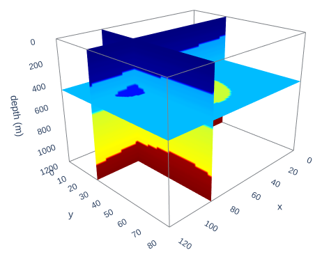
Above is the 3-D velocity model behind that modelling run, viewed with
axes=('x','y','depth'); property volumes get depth labels and min/max colour
limits automatically.
This tab offers one cuboid and three planes, for a quick look at the volume the gathers live in rather than for volume interpretation. If your data is a volume in the first place, cigvis is the recommended tool: it visualizes 3-D seismic data together with labels, faults, RGT, horizon surfaces, well-log trajectories and curves and geological bodies, and supports 2-D and 1-D data as well, using vispy for 3-D, matplotlib for 2-D/1-D and plotly in Jupyter, with optional viser and OpenVDS backends. The slice view here follows its interaction style.
Display modes and colormaps
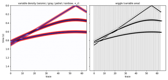
Every 2-D panel switches between variable density and variable-area wiggle.
The sidebar shows the settings of the mode you are in: colormap and
resolution for density, the trace count for wiggle. Flip polarity negates
the display, swapping wiggle fill lobes and density colours together (SEG
normal ↔ reverse). Colormaps are gray (the default), seismic, petrel
(anchors from cigvis), rainbow and viridis, each with an _r reversed
variant. The Clip slider (the clip percentile) sets the colour limits and
doubles as wiggle gain.
Filters and gain
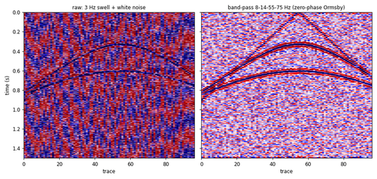
Trapezoid (Ormsby-style) low-pass / high-pass / band-pass filtering:
linear ramps over f1–f2 (low cut) and f3–f4 (high cut), zero phase. Gain
is either AGC (sliding-window RMS, window length editable) or trace
balance. The chain is filter → gain; with gain active the colour limits are
recomputed from the processed gather.
Processing is applied per displayed gather, so memmap laziness is preserved. The Volume slices tab uses the same chain: volumes up to 512 MB are processed whole on each change to the chain, keeping the three planes consistent, while larger memmaps fall back to raw data with a note in the sidebar. If the input is a CuPy array, filtering, gain and picking run on the GPU.
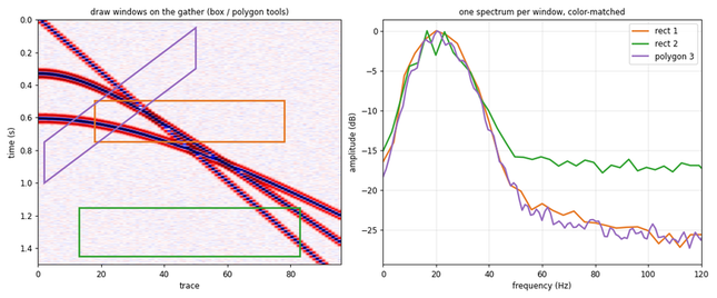
Analysis windows and amplitude spectra
Draw rectangles (SHIFT+drag, or click-move-click) or polygons (click
vertices, ESC to finish) on a gather, then press Compute spectrum: the gated
samples go straight into rfft and |X| is plotted relative to the window's
own peak. No taper, no normalization, no smoothing.
Traces decides how the window's traces reach the plot: Per trace (each
one drawn), Mean (magnitudes averaged) or Middle trace. Scale
switches between Linear amplitude (normalized so the loudest curve peaks at
1.0) and dB. The legend states what was plotted and the frequency spacing
df = 1/(gate length).
Taking no taper has two consequences, both properties of the DFT of a
rectangularly cut record: the boxcar gate's sidelobes fall off only as 1/f, so
roughly 40 dB below the peak what is read is the window rather than the data;
and a single trace's periodogram is a 2-degree-of-freedom estimate whose
scatter does not shrink with record length. Averaging reduces that scatter by
sqrt(N), but only for independent traces — on a coherent gather the traces
are near-copies and the mean differs little from any one of them. A taper
would be a convolution of the spectrum (periodic Hann is (-1/4, 1/2, -1/4)
on the complex spectrum), i.e. smoothing, so none is applied.
Windows export and import as JSON, holding trace/time coordinates and dt.
f-k spectrum
f-k of first window in the Spectrum section transforms the first drawn window in both directions: wavenumber across, frequency up, amplitude in dB relative to the window's own peak over a fixed 60 dB range. A linear event maps to a ray through the origin, so events of different apparent velocity separate, which is what decides whether an apparent-velocity filter is needed and how to set it.
Convention: positive k means events dipping toward increasing trace number.
The axis is in cycles per trace, not per metre — trace spacing is not
necessarily uniform, least of all after an offset or azimuth sort. As with the
1-D spectrum, the transform uses the currently displayed gather, i.e. after the
filter/gain chain, and recomputes when the shot, sort or filter changes. The
window must cover at least 4 traces and 8 samples. Both spectrum panels share
the Panel size selector (S / M / L) and both carry a crosshair and a k / f
readout.
Resolution: what actually reaches the browser
Two controls in the sidebar's Display section decide how much of the gather is drawn, each shown in the mode it applies to, and both say so under the panel when they are thinning it.
Resolution (density mode). Auto caps the image at 1600 pixels per axis — on a 192 x 1250 gather that is no cap at all, and nothing is decimated. Full ships every trace and every sample. The decimation is in pixels: either way the panel spans the whole gather and the axes do not change, so what Auto costs you is detail, not extent.
Traces (wiggle mode). How many traces the wiggle display draws. Raise it for a denser panel, lower it for a cleaner one. Unlike density, this one drops whole traces, so the note appears whenever it is not drawing all of them.
The defaults are budgets, not decisions, because the cost is real:
| gather | auto | full |
|---|---|---|
| 192 x 1250 | 0.2 MB, 0.7 ms | 0.2 MB, 0.5 ms (no cap reached) |
| 960 x 3000 | 1.4 MB, 3.4 ms | 2.9 MB, 3.6 ms |
| 2400 x 4000 | 1.6 MB, 4.6 ms | 9.6 MB, 24 ms |
| 5000 x 12000 | 1.9 MB, 7.3 ms | 60 MB, 200 ms |
That is per redraw, and a redraw happens on every shot step. Up to a few
thousand traces full is free; past that it is a choice worth making
deliberately, which is why it is a control rather than a constant.
Full image is unaffected by either — it always re-renders at one pixel per trace and per sample.
Full-resolution export
Panels are stride-decimated to a pixel budget before going on the wire, and bokeh's save tool snapshots the canvas at its current on-screen size; neither gives the data at its own resolution. The Full image button at the right end of the toolbar row, next to fit and fullscreen, re-renders the gather at one pixel per trace and per sample and downloads a lossless PNG, with colormap, display mode, clip percentile, polarity, filter and gain as displayed. Wiggle mode draws every trace, not the subset the browser receives. The PNG is written by numpy and stdlib zlib, with no matplotlib or headless browser involved.
For a crop of the current view, use the toolbar's save icon.
The same from a script, for batch figures:
from gathervis.process import bandpass, agc
from gathervis.render import save_png

a = agc(bandpass(g.shot(7), g.dt, f3=60, f4=80), g.dt)
save_png("shot007.png", a, cmap="gray")            # or display="wiggle"
First-break and event picking
The pick tool in the plot toolbar adds a pick on tap, moves one on drag and deletes the selected one on BACKSPACE. A dotted line connects the picks in trace order. Auto pick in the First breaks section runs a gapped STA/LTA first-break picker on the currently displayed (i.e. filtered) gather, with STA, LTA and trigger ratio editable: the LTA window ends where the STA window starts, so a break arriving early in the record can still trigger, and a trigger must hold for about STA/2 to exclude single-sample noise. Snap, in Event picking, moves a pick to the nearest peak, trough or |max| of its own trace, searching ±30 ms.
Picks are stored per shot and follow the shot being browsed. They are keyed to
the trace rather than the screen column, so they still match after a re-sort.
Export and import as CSV, shot,trace,time_s.
SEG-Y import
gv.from_segy('field.sgy'), or gathervis field.sgy from the shell. dt is
read from the binary header, traces are grouped into shots by field record
number (FFID), and source and receiver coordinates are read from the standard
trace-header words and scaled by the SEG-Y coordinate scalar rule, so the
The Geometry tab, fold map included, is immediately usable. Shots with unequal trace counts
are zero-padded and a warning is printed. Requires the optional segyio
package; the file is read into memory, and one estimated above max_gb
(8 GB by default) is refused.
Remote usage
- VS Code Remote-SSH (recommended). Run any example in the integrated
terminal; VS Code auto-forwards the port and the printed
http://localhost:8080becomes clickable. Zero setup. - Jupyter. Omit
port=and the returned app renders inline in the notebook — no extra port at all. - Bare terminal.
ssh -L 8080:localhost:8080 user@gpu-server, then open the URL locally. If the port is busy gathervis auto-picks a free one and prints it.
The page loads nothing from the internet: no web fonts, no CDN scripts or icons. It opens as fast on an air-gapped cluster, or from a network where those hosts are slow or blocked, as it does anywhere else. Each browser tab is a session of its own, so colleagues on the same server do not move each other's shots, and a shared link opens exactly the view it describes.
Array semantics
The last axis is always the vertical one: time for data, depth for
property volumes. A bare 3-D array defaults to (shot, rec, time) and is
browsed shot by shot; a 4-D array defaults to (shot, recy, recx, time), one
3-D shot record per shot. Pass view='slices' to slice a 3-D array as a
volume instead, or declare other semantics explicitly with axes=. axes
says what the array is, view says how to look at it, and sort (in the
app) says in what order — the three are independent.
Design notes
- Lazy loading. Data opens as a memmap; browsing a shot reads only that shot's bytes, slicing reads only that slice, and filtering and spectra apply to the displayed gather only. Sorting by acquisition order or receiver line is lazy too (a reshape, a slice); only offset/azimuth order materialises the shot — one shot, not the file.
- Wire format. Panels are stride-decimated to a pixel budget and quantized to uint8 server-side before being sent to the browser.
- Ordering separate from processing. A sort only changes trace order and returns the shot's own traces; the filter/gain chain then runs on the result, so 2-D and 3-D shots share one processing path.
- Two rendering paths. 2-D panels are bokeh images or wiggles, volumes are plotly WebGL slice planes, both fed by the same decimate → uint8 pipeline.
- Export path independent of display. Image export bypasses decimation: the same processed array is rasterized at native resolution and encoded as a PNG with numpy and stdlib zlib, adding no plotting or imaging dependency.
- One look, in one place.
gathervis/theme.pyholds the design (a Panel design plus one stylesheet for every widget), the page template and the figure style; the viewer code says what is on screen, the theme what it looks like. System fonts, one accent colour used only for state. - One session per browser tab. A bokeh model belongs to exactly one document, so every session builds its own workspace over the same (lazy) data rather than sharing figures.
- Interaction state preserved. Sliders update while dragging; the 3-D camera, stretch factors and drawn windows survive updates. Every 2-D panel has x-only / y-only wheel zoom and a client-side cursor readout (trace, time, amplitude under the mouse); the spectrum panels have the same readout and a toggleable crosshair.
Roadmap
M2 (remaining): synced comparison panels · client-side volume cache for
cigvis-grade slice scrubbing (AGC / trace balance / CuPy: done). 3-D
acquisition QC (remaining): shot-record time slices over the receiver grid ·
offset-azimuth rose diagrams per bin (3-D shot sorting, CMP fold map: done). M3 (remaining): header indexing, gather extraction by any key
(SEG-Y import: done). M4 (remaining):
common-offset/time slicing (event picking, NMO preview, velocity spectra and
hand-picked velocity analysis: done). Full plan:
docs/plan.md. And whatever you ask for — see the note at
the top.
Acknowledgements
The velocity-analysis method was taught to me by Prof. Gerard Schuster at an SEG course in Chengdu in 2025. I am very grateful to him. The automatic K-means picker built on it lives in kmeans-vel-picker; what is here is hand picking, because deciding is the person's job.
The petrel colormap anchors come from
cigvis (MIT). Modelling examples use
deepwave. Built on
Panel, Bokeh and
Plotly.
License
MIT
1 maintainer

Metadata
1 maintainer
Release files for gathervis 0.16.0
For a detailed explanation of source distributions (sdists) and built distributions (wheels), please see the package formats documentation.
Source distribution (sdist)
| File | Size | Uploaded | |
|---|---|---|---|
| gathervis-0.16.0.tar.gz | 206.8 kB | Details |
Built distribution (wheel)
| File | Interpreter | ABI | Platform | Reset |
|---|---|---|---|---|
| gathervis-0.16.0-py3-none-any.whl | Python 3 | none | any | Details |
Total release size: 329.3 kB
Release files / gathervis-0.16.0.tar.gz
| Download URL | gathervis-0.16.0.tar.gz |
|---|---|
| Size | 206.8 kB |
| Tags | Source |
|
SHA-256 checksum How to use checksums |
df21b529262c2dc7592e351bc7194414fa239e49dad76b15492405cbaca60e7f
|
|
BLAKE2b-256 checksum How to use checksums |
ec861e72bcc0ef5466256c9008e9b91327d3679cd3f82ccd9f1c0361c45251f5
|
| Upload date | |
|
Uploaded using Trusted Publishing? What is trusted publishing? |
Yes |
| Uploaded via |
twine/7.0.0 CPython/3.13.14
|
Provenance
Provenance describes where a file came from. On PyPI, provenance is shared via attestations, which provide a verifiable record of the build or publishing details. View details, limitations and caveats.


PyPI Publish Attestation
PyPI verified that this artifact, at this checksum, originated from the publisher listed below.
Signed by GitHub Actions, verified by PyPI on Sep 24, 2026.
Transparency logRelease files / gathervis-0.16.0-py3-none-any.whl
| Download URL | gathervis-0.16.0-py3-none-any.whl |
|---|---|
| Size | 122.5 kB |
| Tags | Python 3 |
|
SHA-256 checksum How to use checksums |
cee4e50e56fc3b6dfaf704a3957dea82da57d0ccd9352782b89d664a68642136
|
|
BLAKE2b-256 checksum How to use checksums |
aeacf5b0b20fbbd8db208d7e340edfe91d0b6c4d8472f67a179a81719c4f8b17
|
| Upload date | |
|
Uploaded using Trusted Publishing? What is trusted publishing? |
Yes |
| Uploaded via |
twine/7.0.0 CPython/3.13.14
|
Provenance
Provenance describes where a file came from. On PyPI, provenance is shared via attestations, which provide a verifiable record of the build or publishing details. View details, limitations and caveats.
PyPI Publish Attestation
PyPI verified that this artifact, at this checksum, originated from the publisher listed below.
Signed by GitHub Actions, verified by PyPI on Sep 24, 2026.
Transparency log












