GEDSpy (Gene Enrichment for Drug Searching)

Project description
GEDSpy (Gene Enrichment for Drug Searching) - python library


GEDSpy is the python library for gene list enrichment with genes ontology, pathways, tissue & cell type specificity, genes interactions and cell connections

Author: Jakub Kubiś
Polish Academy of Sciences
Description
GEDSpy is a Python library designed for the analysis of biological data, particularly in high-throughput omics studies. It is a powerful tool for RNA-seq, single-cell RNA-seq, proteomics, and other large-scale biological analyses where numerous differentially expressed genes or proteins are identified. GEDSpy leverages multiple renowned biological databases to enhance functional analysis, pathway enrichment, and interaction studies. It integrates data from: Gene Ontology (A structured framework for gene function classification) , Kyoto Encyclopedia of Genes and Genomes (A resource for understanding high-level functions and utilities of biological systems), Reactome (A curated knowledge base of biological pathways), Human Protein Atlas (A comprehensive database of human protein expression), NCBI (A vast repository of genetic and biomedical data), STRING (A database of known and predicted protein-protein interactions), IntAct (A repository of molecular interaction data), CellTalk (A database for intercellular communication analysis), CellPhone (A tool for inferring cell-cell interactions from single-cell transcriptomics), Human Diseases (A resource linking genes to diseases), ViMic (A database for microbial virulence factors).
GEDSpy is designed to streamline biological data interpretation, enabling researchers to perform in-depth functional analyses, pathway enrichment, and drug target discovery. Its integration of multiple databases makes it an essential tool for translational research, biomarker identification, and disease mechanism exploration.
In this approach, the genomes of Rattus norvegicus and Mus musculus were integrated under the aegis of Homo sapiens, using reference genomes and data from NCBI. This unified genome served as a foundation for mapping data from all utilized datasets. Finally, dedicated algorithms for data analysis were developed and implemented as the GEDSpy library. This advancement simplifies translation studies between the most common animal models and Homo sapiens, facilitating both preclinical and clinical research.
Included data bases:
- Gene Ontology (GO-TERM)
- KEGG (Kyoto Encyclopedia of Genes and Genomes)
- Reactome
- HPA (Human Protein Atlas)
- NCBI
- STRING
- IntAct
- CellTalk
- CellPhone
- Human Diseases
- ViMic
If you use GEDSpy, please remember to cite both GEDSpy and the original sources of the data you utilized in your work.
In the case of enrichment analysis, it is recommended to use the JVectorGraph library to easily adjust and customise graph and network visualisations from the Python side.
Table of contents
-
Enrichment
1.1 Find features in GEDS database
1.2 Enrichment options
1.2.1 Human Protein Atlas (HPA)
1.2.2 Kyoto Encyclopedia of Genes and Genomes (KEGG)
1.2.3 GeneOntology (GO-TERM)
1.2.4 Reactome
1.2.5 Human Diseases
1.2.6 Viral Diseases (ViMIC)
1.2.7 IntAct
1.2.8 STRING
1.2.9 CellConnections
1.2.10 RNAseq of tissues
1.2.11 Full Gene Set Enrichment -
Single Gene Set Analysis (Analysis)
2.1 Set parameters
2.1.1 Interaction parameters
2.1.2 Network parameters
2.1.3 GO-TERM gradation parameter
2.2 Overrepresentation analysis
2.2.1 GO-TERM overrepresenation analysis
2.2.2 KEGG overrepresentation analysis
2.2.3 Reactome overrepresentation analysis
2.2.4 Viral diseases (ViMIC) overrepresentation analysis
2.2.5 Human Diseases overrepresentation analysis
2.2.6 Specificity (HPA) overrepresentation analysis
2.3 Gene Interactions (GI) analysis
2.4 Network analysis
2.4.1 Reactome network analysis
2.4.2 KEGG network analysis
2.4.3 GO-TERM network analysis
2.5 Full enrichment data analysis -
Single Gene Set Visualisation
3.1 Gene type - pie chart
3.2 GO-TERMS - bar plot
3.3 KEGG - bar plot
3.4 Reactome - bar plot
3.5 Specificity - bar plot
3.6 Human Diseases - bar plot
3.7 Viral Diseases (ViMIC) - bar plot
3.8 Blood markers - bar plot
3.9 GOPa - network
3.10 Genes Interactions (GI) - network
3.11 GOPa AutoML - network
3.12 RNAseq tissue - scatter plot -
Differential Set Analysis (DSA)
4.1 DSA - FC parameter
4.2 GO-TERM - DSA
4.3 KEGG - DSA
4.4 Reactome - DSA
4.5 Specificity (HPA) - DSA
4.6 Genes Interactions (GI) - DSA
4.7 Network analysis - DSA
4.8 Inter CellConnection (ICC)
4.9 Inter Terms (IT) - DSA
4.10 Full analysis - DSA -
Differential Set Analysis (DSA) Visualisation
5.1 Both sets graphs
5.1.1 Gene type - pie chart
5.1.2 GO-TERMS - bar plot
5.1.3 KEGG - bar plot
5.1.4 Reactome - bar plot
5.1.5 Specificity - bar plot
5.1.6 Human Diseases - bar plot
5.1.7 Viral Diseases (ViMIC) - bar plot
5.1.8 GOPa - network
5.1.9 Genes Interactions (GI) - network
5.1.10 GOPa AutoML - network
5.1.11 RNAseq tissue - scatter plot
5.1.12 Adjusted Terms - Heatmap -
GetRawData
6.1 Get combined genome
6.2 Get annotated RNAseq data
6.3 Get annotated Reactome data
6.4 Get annotated HPA data
6.5 Get annotated Human Diseases data
6.6 Get annotated viral diseases (ViMIC) data
6.7 Get annotated KEGG data
6.8 Get annotated GO-TERM data
6.9 Get annotated IntAct data
6.10 Get annotated STRING data
6.11 Get adjusted CellTalk data
6.12 Get adjusted CellPhone data
6.13 Get annotated CellInteraction data -
GetRawData
7.1 Get combined genome
7.2 Get RNAseq data
7.3 Get raw Reactome data
7.4 Get raw HPA data
7.5 Get raw Human Diseases data
7.6 Get raw viral diseases (ViMIC) data
7.7 Get raw KEGG data
7.8 Get raw GO-TERM data
7.9 Get raw IntAct data
7.10 Get raw STRING data
7.11 Get raw CellTalk data
7.12 Get raw CellPhone data -
DataDownloading
8.1 Reference genome
8.2 RNAseq data
8.3 IntAct data
8.4 Human diseases data
8.5 Viral diseases data
8.6 Human Protein Atlas - tissue / cell data
8.7 STRING - interaction data
8.8 KEGG data
8.9 REACTOME data
8.10 GO-TERM data
8.11 CellTalk data
8.12 CellPhone data -
UpdatePanel
9.1 Check last update of data
9.2 Update data from GEDSdb
9.3 Update data from data sources
Installation
In command line write:
pip install gedspy
Usage
1. Enrichment
The data sets are annotated to the Ref_Genome (get_REF_GEN()) by ids
from gedspy import Enrichment

# initiate class
enr = Enrichment()
1.1 Find features in GEDS database
- Homo sapiens / Mus musculus / Rattus norvegicus
enr.select_features(features_list)
This method searches for the occurrence of genes or proteins in the GEDS database.
Available names include those from HGNC, Ensembl, or NCBI gene names or IDs,
for the species Homo sapiens, Mus musculus, or Rattus norvegicus.

    Args:
        features_list (list) - list of features (gene or protein names or IDs)

    Returns:
        Updates `self.genome` with feature information found in the GEDS database
1.2 Enrichment options
1.2.1 Human Protein Atlas (HPA)
enr.enriche_specificiti()
This method selects elements from the GEDS database that are included in the Human Protein Atlas (HPA) information.
It includes specificity to the following categories:
    - HPA_RNA_tissue
    - HPA_RNA_single_cell
    - HPA_RNA_cancer
    - HPA_RNA_brain
    - HPA_RNA_blood
    - HPA_RNA_blood_lineage
    - HPA_RNA_cell_line
    - HPA_RNA_mouse_brain_region
    - HPA_subcellular_location
    - HPA_blood_markers

    Returns:
        Updates `self.HPA` with Human Protein Atlas information.
        To retrieve the results, use the `self.get_HPA` method.
HPA_data = enr.get_HPA
This method returns the Human Protein Atlas (HPA) information.
It includes specificity to the following categories:
    - HPA_RNA_tissue
    - HPA_RNA_single_cell
    - HPA_RNA_cancer
    - HPA_RNA_brain
    - HPA_RNA_blood
    - HPA_RNA_blood_lineage
    - HPA_RNA_cell_line
    - HPA_RNA_mouse_brain_region
    - HPA_subcellular_location
    - HPA_blood_markers

    Returns:
        Returns `self.HPA` with Human Protein Atlas information enriched using the `self.enriche_specificiti` method.
1.2.2 Kyoto Encyclopedia of Genes and Genomes (KEGG)
enr.enriche_KEGG()
This method selects elements from the GEDS database that are included in the Kyoto Encyclopedia of Genes and Genomes (KEGG) information.

    Returns:
        Updates `self.KEGG` with KEGG information.
        To retrieve the results, use the `self.get_KEGG` method.
KEGG_data = enr.get_KEGG
This method returns the Kyoto Encyclopedia of Genes and Genomes (KEGG) information.

    Returns:
        Returns `self.KEGG` with KEGG information enriched using the `self.enriche_KEGG` method.
1.2.3 GeneOntology (GO-TERM)
enr.enriche_GOTERM()
This method selects elements from the GEDS database that are included in the GeneOntology (GO-TERM) information.

    Returns:
        Updates `self.GO` with GO-TERM information.
        To retrieve the results, use the `self.get_GO_TERM` method.
GO_data = enr.get_GO_TERM
This method returns the GeneOntology (GO-TERM) information.

    Returns:
        Returns `self.GO` with GeneOntology (GO-TERM) information enriched using the `self.enriche_GOTERM` method.
1.2.4 Reactome
enr.enriche_REACTOME()
This method selects elements from the GEDS database that are included in the Reactome information.

    Returns:
        Updates `self.REACTOME` with Reactome information.
        To retrieve the results, use the `self.get_REACTOME` method.
REACTOME_data = enr.get_REACTOME
This method returns the Reactome information.

    Returns:
        Returns `self.REACTOME` with Reactome information enriched using the `self.enriche_REACTOME` method.
1.2.5 Human Diseases
enr.enriche_DISEASES()
This method selects elements from the GEDS database that are included in the Human Diseases information.

    Returns:
        Updates `self.Diseases` with Human Diseases information.
        To retrieve the results, use the `self.get_DISEASES` method.
DISEASES_data = enr.get_DISEASES
This method returns the Human Diseases information.

    Returns:
        Returns `self.Diseases` with Human Diseases information enriched using the `self.enriche_DISEASES` method.
1.2.6 Viral Diseases (ViMIC)
enr.enriche_ViMIC()
This method selects elements from the GEDS database that are included in the Viral Diseases (ViMIC) information.

    Returns:
        Updates `self.ViMIC` with Viral Disease (ViMIC) information.
        To retrieve the results, use the `self.get_ViMIC` method.
ViMIC_data = enr.get_ViMIC
This method returns the Viral Diseases (ViMIC) information.

    Returns:
        Returns `self.ViMIC` with Viral Diseases (ViMIC) information enriched using the `self.enriche_ViMIC` method.
1.2.7 IntAct
enr.enriche_IntAct()
This method selects elements from the GEDS database that are included in the IntAct information.
It includes specificity to the following data sets:
    - Affinomics
    - Alzheimers
    - BioCreative
    - Cancer
    - Cardiac
    - Chromatin
    - Coronavirus
    - Cyanobacteria
    - Diabetes
    - Huntington
    - IBD
    - Neurodegeneration
    - Parkinsons
    - Rare Diseases
    - Ulcerative

    Returns:
        Updates `self.IntAct` with IntAct information.
        To retrieve the results, use the `self.get_IntAct` method.
IntAct_data = enr.get_IntAct
This method returns the IntAct information.
It includes specificity to the following data sets:
    - Affinomics
    - Alzheimers
    - BioCreative
    - Cancer
    - Cardiac
    - Chromatin
    - Coronavirus
    - Cyanobacteria
    - Diabetes
    - Huntington
    - IBD
    - Neurodegeneration
    - Parkinsons
    - Rare Diseases
    - Ulcerative

    Returns:
        Returns `self.IntAct` with IntAct information enriched using the `self.enriche_IntAct` method.
1.2.8 STRING
enr.enriche_STRING()
This method selects elements from the GEDS database that are included in the STRING information.

    Returns:
        Updates `self.STRING` with STRING information.
        To retrieve the results, use the `self.get_STRING` method.
STRING_data = enr.get_STRING
This method returns the STRING information.

    Returns:
        Returns `self.STRING` with STRING information enriched using the `self.enriche_STRING` method.
1.2.9 CellConnections
enr.enriche_CellCon()
This method selects elements from the GEDS database that are included in the CellPhone / CellTalk information.

    Returns:
        Updates `self.CellCon` with CellPhone / CellTalk information.
        To retrieve the results, use the `self.get_CellCon` method.
CellCon_data = enr.get_CellCon
This method returns the CellPhone / CellTalk information.

    Returns:
        Returns `self.CellCon` with Human Protein Atlas information enriched using the `self.enriche_CellCon` method.
1.2.10 RNAseq of tissues
enr.enriche_RNA_SEQ()
This method selects elements from the GEDS database that are included in the RNAseq information.
It includes specificity to the following data sets:
    -human_tissue_expression_HPA
    -human_tissue_expression_RNA_total_tissue
    -human_tissue_expression_fetal_development_circular

    Returns:
        Updates `self.RNA_SEQ` with RNAseq information.
        To retrieve the results, use the `self.get_RNA_SEQ` method.
RNASEQ_data = enr.get_RNA_SEQ
This method returns the RNAseq information.
It includes specificity to the following data sets:
    -human_tissue_expression_HPA
    -human_tissue_expression_RNA_total_tissue
    -human_tissue_expression_fetal_development_circular

    Returns:
        Returns `self.RNA_SEQ` with RNAseq information enriched using the `self.enriche_RNA_SEQ` method.
1.2.11 Full Gene Set Enrichment
enr.full_enrichment()
This method conducts a full enrichment analysis based on the GEDS database, which includes:
    - Human Protein Atlas (HPA) [see self.enriche_specificiti() method]
    - Kyoto Encyclopedia of Genes and Genomes (KEGG) [see self.enriche_KEGG() method]
    - GeneOntology (GO-TERM) [see self.enriche_GOTERM() method]
    - Reactome [see self.enriche_REACTOME() method]
    - Human Diseases [see self.enriche_DISEASES() method]
    - Viral Diseases (ViMIC) [see self.enriche_ViMIC() method]
    - IntAct [see self.enriche_IntAct() method]
    - STRING [see self.enriche_STRING() method]
    - CellConnections (CellPhone / CellTalk) [see self.enriche_CellCon() method]
    - RNAseq data specific to tissues [see self.enriche_RNA_SEQ() method]

    Returns:
        To retrieve the results, use the `self.get_results` method.
results = enr.get_results()
This method returns the full enrichment analysis dictionary containing on keys:
    - 'gene_info' - genome information for the selected gene set [see `self.get_gene_info` property]
    - 'HPA' - Human Protein Atlas (HPA) [see 'self.get_HPA' property]
    - 'KEGG' - Kyoto Encyclopedia of Genes and Genomes (KEGG) [see 'self.get_KEGG' property]
    - 'GO-TERM' - GeneOntology (GO-TERM) [see 'self.get_GO_TERM' property]
    - 'REACTOME' - Reactome [see 'self.get_REACTOME' property]
    - 'DISEASES' - Human Diseases [see 'self.get_DISEASES' property]
    - 'ViMIC' - Viral Diseases (ViMIC) [see 'self.get_ViMIC' property]
    - 'IntAct' - IntAct [see 'self.get_IntAct' property]
    - 'STRING' - STRING [see 'self.get_STRING' property]
    - 'CellConnections' - CellConnections (CellPhone / CellTalk) [see 'self.get_CellCon' property]
    - 'RNA-SEQ' - RNAseq data specific to tissues [see 'self.get_RNA_SEQ' property]

    Returns:
        dict (dict) - full enrichment data
2. Single Gene Set Analysis
from gedspy import Analysis

# initiate class
ans = Analysis(input_data)
The `Analysis` class provides tools for statistical and network analysis of `Enrichment` class results obtained using the `self.get_results` method.

    Args:
        input_data (dict) - output data from the `Enrichment` class `self.get_results` method
2.1 Set parameters
2.1.1 Interaction parameters
ans.interactions_metadata
This method returns current interactions parameters:

    -interaction_strength : int - value of enrichment strenght for STRING data:
        *900 - very high probabylity of interaction;
        *700 - medium probabylity of interaction,
        *400 - low probabylity of interaction,
        *<400 - very low probabylity of interaction


    -interaction_source : list - list of sources for interaction estimation:
        *STRING: ['STRING']
        *IntAct: ['Affinomics', 'Alzheimers','BioCreative', 'Cancer',
                    'Cardiac', 'Chromatin', 'Coronavirus', 'Diabetes',
                    "Huntington's", 'IBD', 'Neurodegeneration', 'Parkinsons']


    Returns:
        dict : {'interaction_strength' : int,
                'interaction_source' : list}
ans.set_interaction_strength(value)
This method sets self.interaction_strength parameter.

    The 'interaction_strength' value is used for enrichment strenght of STRING data:
         *900 - very high probabylity of interaction;
         *700 - medium probabylity of interaction,
         *400 - low probabylity of interaction,
         *<400 - very low probabylity of interaction

    Args:
        value (int) - value of interaction strength
ans.set_interaction_source(sources_list)
This method sets self.interaction_source parameter.

    The 'interaction_source' value is list of sources for interaction estimation:

        *STRING / IntAct: ['STRING', 'Affinomics', 'Alzheimers','BioCreative',
                            'Cancer', 'Cardiac', 'Chromatin', 'Coronavirus',
                            'Diabetes', "Huntington's", 'IBD', 'Neurodegeneration',
                            'Parkinsons']

    Args:
        sources_list (list) - list of source data for interactions network analysis
2.1.2 Network parameters
ans.networks_metadata
This method returns current networks creation parameters:

    -test : str - test type for enrichment overrepresentation analysis.
        Available test:
            *BIN - binomial test
            *FISH - Fisher's exact test

    -adj : str | None - p_value correction.
        Available correction:
            *BF - Bonferroni correction
            *BH - Benjamini-Hochberg correction
            *None - lack of correction

    -p_val : float - threshold for p-value in network creation


    Returns:
        dict : {'test': str,
                'adj': str | None,
                'p_val': float}
ans.set_p_value(value)
This method sets the p-value threshold for network creation

    Args:
        value (float) - p-value threshold for network creation
ans.set_test(test)
This method sets the statistical test to be used for network creation.

        Avaiable tests:
            - 'FISH' - Fisher's exact test
            - 'BIN' - Binomial test

        Args:
            test (str) - test acronym ['FISH'/'BIN']
ans.set_correction(correction)
This method sets the statistical test correction to be used for network creation.

    Avaiable tests:
        - 'BF' - Bonferroni correction
        - 'BH' - Benjamini-Hochberg correction
        - None - lack of correction

    Args:
        correction (str / None) - test correction acronym ['BF'/'BH'/None]
2.1.3 GO-TERM gradation parameter
ans.set_go_grade(grade)
 This method sets self.go_grade parameter.

 The 'go_grade' value is used for GO-TERM data gradation [1-4].

        Args:
            grade (int) - grade level for GO terms analysis. Default: 1
2.2 Overrepresentation analysis
2.2.1 GO-TERM overrepresenation analysis
ans.GO_overrepresentation()
This method conducts an overrepresentation analysis of Gene Ontology (GO-TERM) information.

    Returns:
        Updates `self.GO_stat` with overrepresentation statistics for GO-TERM information.
        To retrieve the results, use the `self.get_GO_statistics` method.
GO_results = ans.get_GO_statistics
This method returns the GO-TERM overrepresentation statistics.

    Returns:
        Returns `self.GO_stat` contains GO-TERM overrepresentation statistics obtained using the `self.GO_overrepresentation` method.
2.2.2 KEGG overrepresentation analysis
ans.KEGG_overrepresentation()
This method conducts an overrepresentation analysis of Kyoto Encyclopedia of Genes and Genomes (KEGG) information.

    Returns:
        Updates `self.KEGG_stat` with overrepresentation statistics for KEGG information.
        To retrieve the results, use the `self.get_KEGG_statistics` method.
KEGG_results = ans.get_KEGG_statistics
This method returns the KEGG overrepresentation statistics.

    Returns:
        Returns `self.KEGG_stat` contains KEGG overrepresentation statistics obtained using the `self.KEGG_overrepresentation` method.
2.2.3 Reactome overrepresentation analysis
ans.REACTOME_overrepresentation()
This method conducts an overrepresentation analysis of Reactome information.

    Returns:
        Updates `self.REACTOME_stat` with overrepresentation statistics for Reactome information.
        To retrieve the results, use the `self.get_REACTOME_statistics` method.
REACTOME_results = ans.get_REACTOME_statistics
This method returns the Reactome overrepresentation statistics.

    Returns:
        Returns `self.REACTOME_stat` contains Reactome overrepresentation statistics obtained using the `self.REACTOME_overrepresentation` method.
2.2.4 Viral diseases (ViMIC) overrepresentation analysis
ans.ViMIC_overrepresentation()
This method conducts an overrepresentation analysis of viral diseases ViMIC information.

    Returns:
        Updates `self.ViMIC_stat` with overrepresentation statistics for ViMIC information.
        To retrieve the results, use the `self.get_ViMIC_statistics` method.
ViMIC_results = ans.get_ViMIC_statistics
This method returns the ViMIC overrepresentation statistics.

    Returns:
        Returns `self.ViMIC_stat` contains ViMIC overrepresentation statistics obtained using the `self.ViMIC_overrepresentation` method.
2.2.5 Human Diseases overrepresentation analysis
ans.DISEASES_overrepresentation()
This method conducts an overrepresentation analysis of Human Diseases information.

    Returns:
        Updates `self.DISEASE_stat` with overrepresentation statistics for Human Diseases information.
        To retrieve the results, use the `self.get_DISEASE_statistics` method.
DISEASES_results = ans.get_DISEASE_statistics
This method returns the Human Diseases overrepresentation statistics.

    Returns:
        Returns `self.DISEASE_stat` contains Human Diseases overrepresentation statistics obtained using the `self.DISEASES_overrepresentation` method.
2.2.6 Specificity (HPA) overrepresentation analysis
ans.features_specificity()
 This method conducts an overrepresentation analysis of tissue specificity on Human Protein Atlas (HPA) information.

    Returns:
        Updates `self.specificity_stat` with overrepresentation statistics for specificity information.
        To retrieve the results, use the `self.get_specificity_statistics` method.
specificity_results = ans.get_specificity_statistics
This method returns the tissue specificity [Human Protein Atlas (HPA)] overrepresentation statistics.

    Returns:
        Returns `self.specificity_stat` contains specificity overrepresentation statistics obtained using the `self.features_specificity` method.
2.3 Gene Interactions (GI) analysis
ans.gene_interaction()
This method conducts an Genes Interaction (GI) analysis of STRING / IntAct information.

    Returns:
        Updates `self.features_interactions` with overrepresentation statistics for GI information.
        To retrieve the results, use the `self.get_features_interactions_statistics` method.
GI_results = ans.get_features_interactions_statistics
This method returns the Genes Interactions (GI) data.

    Returns:
        Returns `self.features_interactions` contains GI data obtained using the `self.gene_interaction` method.
2.4 Network analysis
2.4.1 Reactome network analysis
ans.REACTOME_network()
This method conducts an network analysis of Reactome data.

    Returns:
        Updates `self.REACTOME_net` with Reactome network data.
        To retrieve the results, use the `self.get_REACTOME_network` method.
Reactome_network = ans.get_REACTOME_network
This method returns the Reactome network analysis results.

    Returns:
        Returns `self.REACTOME_net` contains Reactome network analysis results obtained using the `self.REACTOME_network` method.
2.4.2 KEGG network analysis
ans.KEGG_network()
 This method conducts an network analysis of KEGG data.

    Returns:
        Updates `self.KEGG_net` with Reactome network data.
        To retrieve the results, use the `self.get_KEGG_network` method.
KEGG_network = ans.get_KEGG_network
This method returns the KEGG network analysis results.

    Returns:
        Returns `self.KEGG_net` contains KEGG network analysis results obtained using the `self.KEGG_network` method.
2.4.3 GO-TERM network analysis
ans.GO_network()
This method conducts an network analysis of GO-TERM data.

    Returns:
        Updates `self.GO_net` with GO-TERM network data.
        To retrieve the results, use the `self.get_GO_network` method.
GO_network = ans.get_GO_network
This method returns the GO-TERM network analysis results.

    Returns:
        Returns `self.GO_net` contains Reactome network analysis results obtained using the `self.GO_network` method.
2.5 Full enrichment data analysis
ans.full_analysis()
This method conducts a full analysis of `Enrichment` class results obtained using the `self.get_results` method:

        * statistics:
            - Human Protein Atlas (HPA) [see self.features_specificity() method]
            - Kyoto Encyclopedia of Genes and Genomes (KEGG) [see self.KEGG_overrepresentation() method]
            - GeneOntology (GO-TERM) [see self.GO_overrepresentation() method]
            - Reactome [see self.REACTOME_overrepresentation() method]
            - Human Diseases [see self.DISEASES_overrepresentation() method]
            - Viral Diseases (ViMIC) [see self.ViMIC_overrepresentation() method]
         * networks:
             - Kyoto Encyclopedia of Genes and Genomes (KEGG) [see self.KEGG_network() method]
             - GeneOntology (GO-TERM) [see self.GO_network() method]
             - Reactome [see self.REACTOME_network() method]


    Returns:
        To retrieve the results, use the `self.get_full_results` method.
full_results = ans.get_full_results
This method returns the full analysis dictionary containing on keys:
        * 'enrichment':
            - 'gene_info' - genome information for the selected gene set [see `self.get_gene_info` property]
            - 'HPA' - Human Protein Atlas (HPA) [see 'self.get_HPA' property]
            - 'KEGG' - Kyoto Encyclopedia of Genes and Genomes (KEGG) [see 'self.get_KEGG' property]
            - 'GO-TERM' - GeneOntology (GO-TERM) [see 'self.get_GO_TERM' property]
            - 'REACTOME' - Reactome [see 'self.get_REACTOME' property]
            - 'DISEASES' - Human Diseases [see 'self.get_DISEASES' property]
            - 'ViMIC' - Viral Diseases (ViMIC) [see 'self.get_ViMIC' property]
            - 'IntAct' - IntAct [see 'self.get_IntAct' property]
            - 'STRING' - STRING [see 'self.get_STRING' property]
            - 'CellConnections' - CellConnections (CellPhone / CellTalk) [see 'self.get_CellCon' property]
            - 'RNA-SEQ' - RNAseq data specific to tissues [see 'self.get_RNA_SEQ' property]

         * 'statistics':
             - 'specificity' - Human Protein Atlas (HPA) [see 'self.get_specificity_statistics' property]
             - 'KEGG' - Kyoto Encyclopedia of Genes and Genomes (KEGG) [see 'self.get_KEGG_statistics' property]
             - 'GO-TERM' - GeneOntology (GO-TERM) [see 'self.get_GO_statistics' property]
             - 'REACTOME' - Reactome [see 'self.get_REACTOME_statistics' property]
             - 'DISEASES' - Human Diseases [see 'self.get_DISEASE_statistics' property]
             - 'ViMIC' - Viral Diseases (ViMIC) [see 'self.get_ViMIC_statistics' property]
             - 'interactions' - STRING / IntAct [see 'self.get_features_interactions_statistics' property]

         * 'networks':
             - 'KEGG' - Kyoto Encyclopedia of Genes and Genomes (KEGG) [see 'self.get_KEGG_network' property]
             - 'GO-TERM' - GeneOntology (GO-TERM) [see 'self.get_GO_network' property]
             - 'REACTOME' - Reactome [see 'self.get_REACTOME_network' property]

    Returns:
        dict (dict) - full analysis data
3. Single Gene Set Visualisation
from gedspy import Visualization

# initiate class
vis = Visualization(input_data)
The `Visualization` class provides tools for statistical and network analysis of `Analysis` class results obtained using the `self.get_full_results` method.

    Args:
        input_data (dict) - output data from the `Analysis` class `self.get_full_results` method
3.1 Gene type - pie chart
plot  =  vis.gene_type_plot(
                cmap = 'summer',
                image_width = 6,
                image_high = 6,
                font_size = 15)
This method generates a pie chart visualizing the distribution of gene types based on enrichment data.

    Args:
        cmap (str) - colormap used for the pie chart. Default is 'summer'
        image_width (int) - width of the plot in inches. Default is 6
        image_high (int) - height of the plot in inches. Default is 6
        font_size (int) - font size. Default is 15

    Returns:
        fig (matplotlib.figure.Figure) - figure object containing a pie chart that visualizes the distribution of gene type occurrences as percentages
3.2 GO-TERMS - bar plot
plot  =  vis.GO_plot(
                p_val = 0.05,
                test = 'FISH',
                adj = 'BH',
                n = 10,
                min_terms = 5,
                selected_parent = [],
                side = 'right',
                color = 'blue',
                width = 10,
                bar_width = 0.5,
                stat = 'p_val')
 This method generates a bar plot for Gene Ontology (GO) term enrichment and statistical analysis.

    Args:
        p_val (float) - significance threshold for p-values. Default is 0.05
        test (str) - statistical test to use ('FISH' - Fisher's Exact Test or 'BIN' - binomial test). Default is 'FISH'
        adj (str) - method for p-value adjustment ('BH' - Benjamini-Hochberg, 'BF' - Benjamini-Hochberg). Default is 'BH'
        n (int) - maximum number of terms to display per category. Default is 25
        min_terms (int) - minimum number of child terms required for a parent term to be included. Default is 5
        selected_parent (list) - list of specific parent terms to include in the plot. If empty, all parent terms are included. Default is []
        side (str) - side on which the bars are displayed ('left' or 'right'). Default is 'right'
        color (str) - color of the bars in the plot. Default is 'blue'
        width (int) - width of the plot in inches. Default is 10
        bar_width (float / int) - width of individual bars. Default is 0.5
        stat (str) - statistic to use for the x-axis ('p_val', 'n', or 'perc'). Default is 'p_val'

    Returns:
        fig (matplotlib.figure.Figure) - matplotlib Figure object containing the bar plots
3.3 KEGG - bar plot
plot  =  vis.KEGG_plot(
                p_val = 0.05,
                test = 'FISH',
                adj = 'BH',
                n = 10,
                min_terms = 5,
                selected_parent = [],
                side = 'right',
                color = 'orange',
                width = 10,
                bar_width = 0.5,
                stat = 'p_val')
This method generates a bar plot for KEGG term enrichment and statistical analysis.

    Args:
        p_val (float) - significance threshold for p-values. Default is 0.05
        test (str) - statistical test to use ('FISH' - Fisher's Exact Test or 'BIN' - binomial test). Default is 'FISH'
        adj (str) - method for p-value adjustment ('BH' - Benjamini-Hochberg, 'BF' - Benjamini-Hochberg). Default is 'BH'
        n (int) - maximum number of terms to display per category. Default is 10
        min_terms (int) - minimum number of child terms required for a parent term to be included. Default is 5
        selected_parent (list) - list of specific parent terms to include in the plot. If empty, all parent terms are included. Default is []
        side (str) - side on which the bars are displayed ('left' or 'right'). Default is 'right'
        color (str) - color of the bars in the plot. Default is 'orange'
        width (int) - width of the plot in inches. Default is 10
        bar_width (float / int) - width of individual bars. Default is 0.5
        stat (str) - statistic to use for the x-axis ('p_val', 'n', or 'perc'). Default is 'p_val'

    Returns:
        fig (matplotlib.figure.Figure) - matplotlib Figure object containing the bar plots
3.4 Reactome - bar plot
plot  =  vis.REACTOME_plot(
                p_val = 0.05,
                test = 'FISH',
                adj = 'BH',
                n = 10,
                min_terms = 5,
                selected_parent = [],
                side = 'right',
                color = 'silver',
                width = 10,
                bar_width = 0.5,
                stat = 'p_val')
This method generates a bar plot for Reactome term enrichment and statistical analysis.

    Args:
        p_val (float) - significance threshold for p-values. Default is 0.05
        test (str) - statistical test to use ('FISH' - Fisher's Exact Test or 'BIN' - binomial test). Default is 'FISH'
        adj (str) - method for p-value adjustment ('BH' - Benjamini-Hochberg, 'BF' - Benjamini-Hochberg). Default is 'BH'
        n (int) - maximum number of terms to display per category. Default is 10
        min_terms (int) - minimum number of child terms required for a parent term to be included. Default is 5
        selected_parent (list) - list of specific parent terms to include in the plot. If empty, all parent terms are included. Default is []
        side (str) - side on which the bars are displayed ('left' or 'right'). Default is 'right'
        color (str) - color of the bars in the plot. Default is 'silver'
        width (int) - width of the plot in inches. Default is 10
        bar_width (float / int) - width of individual bars. Default is 0.5
        stat (str) - statistic to use for the x-axis ('p_val', 'n', or 'perc'). Default is 'p_val'

    Returns:
        fig (matplotlib.figure.Figure) - matplotlib Figure object containing the bar plots
3.5 Specificity - bar plot
plot  =  vis.SPECIFICITY_plot(
                p_val = 0.05,
                test = 'FISH',
                adj = 'BH',
                n = 5,
                side = 'right',
                color = 'bisque',
                width = 10,
                bar_width = 0.5,
                stat = 'p_val')
This method generates a bar plot for tissue specificity [Human Protein Atlas (HPA)] enrichment and statistical analysis.

    Args:
        p_val (float) - significance threshold for p-values. Default is 0.05
        test (str) - statistical test to use ('FISH' - Fisher's Exact Test or 'BIN' - binomial test). Default is 'FISH'
        adj (str) - method for p-value adjustment ('BH' - Benjamini-Hochberg, 'BF' - Benjamini-Hochberg). Default is 'BH'
        n (int) - maximum number of terms to display per category. Default is 5
        side (str) - side on which the bars are displayed ('left' or 'right'). Default is 'right'
        color (str) - color of the bars in the plot. Default is 'bisque'
        width (int) - width of the plot in inches. Default is 10
        bar_width (float / int) - width of individual bars. Default is 0.5
        stat (str) - statistic to use for the x-axis ('p_val', 'n', or 'perc'). Default is 'p_val'

    Returns:
        fig (matplotlib.figure.Figure) - matplotlib Figure object containing the bar plots
3.6 Human Diseases - bar plot
plot  =  vis.DISEASES_plot(
                p_val = 0.05,
                test = 'FISH',
                adj = 'BH',
                n = 5,
                side = 'right',
                color = 'thistle',
                width = 10,
                bar_width = 0.5,
                stat = 'p_val')
This method generates a bar plot for Human Diseases enrichment and statistical analysis.

    Args:
        p_val (float) - significance threshold for p-values. Default is 0.05
        test (str) - statistical test to use ('FISH' - Fisher's Exact Test or 'BIN' - binomial test). Default is 'FISH'
        adj (str) - method for p-value adjustment ('BH' - Benjamini-Hochberg, 'BF' - Benjamini-Hochberg). Default is 'BH'
        n (int) - maximum number of terms to display per category. Default is 5
        side (str) - side on which the bars are displayed ('left' or 'right'). Default is 'right'
        color (str) - color of the bars in the plot. Default is 'thistle'
        width (int) - width of the plot in inches. Default is 10
        bar_width (float / int) - width of individual bars. Default is 0.5
        stat (str) - statistic to use for the x-axis ('p_val', 'n', or 'perc'). Default is 'p_val'

    Returns:
        fig (matplotlib.figure.Figure) - matplotlib Figure object containing the bar plots
3.7 Viral Diseases (ViMIC) - bar plot
plot  =  vis.ViMIC_plot(
                p_val = 0.05,
                test = 'FISH',
                adj = 'BH',
                n = 5,
                side = 'right',
                color = 'aquamarine',
                width = 10,
                bar_width = 0.5,
                stat = 'p_val')
This method generates a bar plot for Viral Diseases (ViMIC) enrichment and statistical analysis.

    Args:
        p_val (float) - significance threshold for p-values. Default is 0.05
        test (str) - statistical test to use ('FISH' - Fisher's Exact Test or 'BIN' - binomial test). Default is 'FISH'
        adj (str) - method for p-value adjustment ('BH' - Benjamini-Hochberg, 'BF' - Benjamini-Hochberg). Default is 'BH'
        n (int) - maximum number of terms to display per category. Default is 5
        side (str) - side on which the bars are displayed ('left' or 'right'). Default is 'right'
        color (str) - color of the bars in the plot. Default is 'aquamarine'
        width (int) - width of the plot in inches. Default is 10
        bar_width (float / int) - width of individual bars. Default is 0.5
        stat (str) - statistic to use for the x-axis ('p_val', 'n', or 'perc'). Default is 'p_val'

    Returns:
        fig (matplotlib.figure.Figure) - matplotlib Figure object containing the bar plots
3.8 Blood markers - bar plot
plot  =  vis.blod_markers_plot(
                    n = 10,
                    side = 'right',
                    color = 'red',
                    width = 10,
                    bar_width = 0.5)
This method generates a bar plot for Blood Markers enrichment analysis.

    Args:
        p_val (float) - significance threshold for p-values. Default is 0.05
        n (int) - maximum number of terms to display per category. Default is 5
        side (str) - side on which the bars are displayed ('left' or 'right'). Default is 'right'
        color (str) - color of the bars in the plot. Default is 'red'
        width (int) - width of the plot in inches. Default is 10
        bar_width (float / int) - width of individual bars. Default is 0.5

    Returns:
        fig (matplotlib.figure.Figure) - matplotlib Figure object containing the bar plots
3.9 GOPa - network
plot  =  vis.GOPa_network_create(
                            data_set = 'GO-TERM',
                            genes_inc = 10,
                            gene_int = True,
                            genes_only = True,
                            min_con = 2,
                            children_con = False,
                            include_childrend = True,
                            selected_parents = [],
                            selected_genes = [])
This method creates a network graph for Gene Ontology (GO) or pathway analysis.

    Args:
        data_set (str) - type of data set to use for the network ['GO-TERM', 'KEGG', 'REACTOME']. Default is 'GO-TERM'
        genes_inc (int) - number of top genes to include in the network based on their occurrence. Default is 10
        gene_int (bool) - whether to include gene-gene interactions in the network. Default is True
        genes_only (bool) - whether to restrict the network to only include selected genes and their connections. Default is True
        min_con (int) - minimum number of connections required for a GO term or pathway to be included in the network. Default is 2.
        children_con (bool) - whether to include child connections in the network. Default is False
        include_childrend (bool) - whether to include children terms as nodes in the network. Default is True
        selected_parents (list) - specific parent terms to include in the network. If empty, all parents are considered. Default is []
        selected_genes (list) - specific genes to include in the network. If empty, all genes are considered. Default is []

    Returns:
        fig (networkx.Graph) - NetworkX Graph object representing the GO or pathway network
3.10 Genes Interactions (GI) - network
plot = vis.GI_network_create(min_con = 2)
This method creates a gene or protein interaction network graph.

    Args:
        min_con (int) - minimum number of connections (degree) required for a gene or protein to be included in the network. Default is 2

    Returns:
        fig (networkx.Graph) - NetworkX Graph object representing the interaction network, with nodes sized by connection count and edges colored by interaction type
3.11 GOPa AutoML - network
plot  =  vis.AUTO_ML_network(
                        genes_inc = 10,
                        gene_int = True,
                        genes_only = True,
                        min_con = 2,
                        children_con = False,
                        include_childrend = False,
                        selected_parents = [],
                        selected_genes = [])
This method creates a machine learning supported multi-layered network of gene or protein interactions using GO-TERM, KEGG, and REACTOME data.

    Args:
        genes_inc (int) - number of top genes to include based on interaction frequency. Default is 10
        genes_inc (int) - number of top genes to include in the network based on their occurrence. Default is 10
        gene_int (bool) - whether to include gene-gene interactions in the network. Default is True
        genes_only (bool) - whether to restrict the network to only include selected genes and their connections. Default is True
        min_con (int) - minimum number of connections required for a GO term or pathway to be included in the network. Default is 2.
        children_con (bool) - whether to include child connections in the network. Default is False
        include_childrend (bool) - whether to include children terms as nodes in the network. Default is True
        selected_parents (list) - specific parent terms to include in the network. If empty, all parents are considered. Default is []
        selected_genes (list) - specific genes to include in the network. If empty, all genes are considered. Default is []

    Returns
       Returns:
           fig (networkx.Graph) - NetworkX Graph object representing the GO and pathway network
3.12 RNAseq tissue - scatter plot
plot  =  vis.gene_scatter(
                     colors = 'viridis',
                     species = 'human',
                     hclust = 'complete',
                     img_width = None,
                     img_high = None,
                     label_size = None,
                     x_lab = 'Genes',
                     legend_lab = 'log(TPM + 1)',
                     selected_list = [])
Visualizes RNA-SEQ enrichment data using scatter plots with hierarchical clustering.

    RNA-SEQ data including:
       -human_tissue_expression_HPA
       -human_tissue_expression_RNA_total_tissue
       -human_tissue_expression_fetal_development_circular

    Args:
        colors (str) - colormap used for scatter plot points. Default is 'viridis'
        species (str) - determines the case formatting of tissue labels. Use 'human' for uppercase labels, or other values for title case. Default is 'human'
        hclust (str) - hierarchical clustering method applied to reorder rows and columns. Options include 'single', 'complete', 'average', etc. Default is 'complete'
        img_width (int / None) - width of the output image in inches. If None, the width is determined based on the number of genes. Default is None
        img_high (int / None) - height of the output image in inches. If None, the height is determined based on the number of tissues. Default is None
        label_size (int / None) - font size for axis labels and tick marks. Calculated dynamically if None. Default is None
        x_lab (str) - label for the x-axis. Default is 'Genes'
        legend_lab (str,) - label for the color bar legend. Default is 'log(TPM + 1)'
        selected_list (list) - list of specific genes to include in the visualization. If left empty, all genes from the dataset will be displayed. Default is []

    Returns:
        return_dict (dict) - dictionary with dataset names as keys and their corresponding matplotlib figures as values. Each figure shows a scatter plot of the different RNAseq data
4. Differential Set Analysis (DSA)
from gedspy import DSA

# initiate class
dsa_compare = DSA(set1, set2)
The 'DSA' class performs Differential Set Analysis by taking the results from two independent feature lists (e.g., upregulated and downregulated genes).
It utilizes input data derived from independent gene sets obtained through statistical and network analyses, which are part of the Analysis class results.
These results are accessed using the 'self.get_full_results' method.


    Args:
        set1 (dict)- output data from the `Analysis` class `self.get_full_results` method of genes set eg. ['KIT', 'EDNRB', 'PAX3']
        set2 (dict)- output data from the `Analysis` class `self.get_full_results` method of genes set eg. ['MC4R', 'MITF', 'SLC2A4']
4.1 DSA - FC parameter
dsa_compare.set_min_fc(fc)
This method set 'self.min_fc' value, which is necessary for conducting Differential Set Analysis (DSA).
    The value must be numeric and greater than 1.

    Overview:
        The DSA method assesses differences between set1 and set2 by calculating the normalized occurrence ('n_occ') of each term in both sets and determining the Fold Change (FC) between these occurrences.
        For term that is absent in one of sets, their normalized occurrence ('n_occ') is assigned a value equal to half the minimum 'n_occ' observed across all terms within the analysis type (e.g., GO-TERM, KEGG, etc.).
        By analyzing these FC values, the method identifies key differences in enrichment between the two sets, highlighting biologically significant pathways or terms unique or equal to each set.

    Formulas:
        The normalized occurrence ('n_occ') for each term is calculated as:
           n_occ = genes per term / total genes per set

        The Fold Change (FC) is then computed as the ratio of normalized occurrences:
           FC = set1 n_occ / set2 n_occ


    Interpretation:
       - If FC > self.min_fc, the term is considered more enriched in set1
       - If FC < 1/self.min_fc, the term is considered more enriched in set2
       - If FC < self.min_fc and > 1/self.min_fc, the term is equal between sets

    Args:
        fc (float) - Fold Change threshold value to be set. The value must be numeric and greater than 1. Default is 1.5.
4.2 GO-TERM - DSA
dsa_compare.GO_diff()
This method performs a Differential Set Analysis (DSA) to compare two sets (set1 and set2) based on their Gene Ontology (GO-TERM) enrichment analysis.

    Overview:
        This method assesses differences between set1 and set2 by calculating the normalized occurrence ('n_occ') of each term in both sets and determining the Fold Change (FC) between these occurrences.
        For term that is absent in one of sets, their normalized occurrence ('n_occ') is assigned a value equal to half the minimum 'n_occ' observed across all terms within the analysis type (e.g., GO-TERM, KEGG, etc.).
        By analyzing these FC values, the method identifies key differences in enrichment between the two sets, highlighting biologically significant pathways or terms unique or equal to each set.

    Formulas:
        The normalized occurrence ('n_occ') for each term is calculated as:
           n_occ = genes per term / total genes per set

        The Fold Change (FC) is then computed as the ratio of normalized occurrences:
           FC = set1 n_occ / set2 n_occ


    Interpretation:
       - If FC > self.min_fc, the term is considered more enriched in set1
       - If FC < 1/self.min_fc, the term is considered more enriched in set2
       - If FC < self.min_fc and > 1/self.min_fc, the term is equal between sets

    Returns:
        Updates `self.GO` with Reactome DSA data.
        To retrieve the results, use the `self.get_GO_diff` method.
GO_diff_results = ans.get_GO_diff
This method returns the GO-TERM Differential Set Analysis (DSA)

    Returns:
        Returns `self.GO` contains GO-TERM DSA obtained using the `self.GO_diff` method.
4.3 KEGG - DSA
dsa_compare.KEGG_diff()
This method performs a Differential Set Analysis (DSA) to compare two sets (set1 and set2) based on their KEGG enrichment analysis.

    Overview:
        This method assesses differences between set1 and set2 by calculating the normalized occurrence ('n_occ') of each term in both sets and determining the Fold Change (FC) between these occurrences.
        For term that is absent in one of sets, their normalized occurrence ('n_occ') is assigned a value equal to half the minimum 'n_occ' observed across all terms within the analysis type (e.g., GO-TERM, KEGG, etc.).
        By analyzing these FC values, the method identifies key differences in enrichment between the two sets, highlighting biologically significant pathways or terms unique or equal to each set.

    Formulas:
        The normalized occurrence ('n_occ') for each term is calculated as:
           n_occ = genes per term / total genes per set

        The Fold Change (FC) is then computed as the ratio of normalized occurrences:
           FC = set1 n_occ / set2 n_occ


    Interpretation:
       - If FC > self.min_fc, the term is considered more enriched in set1
       - If FC < 1/self.min_fc, the term is considered more enriched in set2
       - If FC < self.min_fc and > 1/self.min_fc, the term is equal between sets

    Returns:
        Updates `self.KEGG` with Reactome DSA data.
        To retrieve the results, use the `self.get_KEGG_diff` method.
KEGG_diff_results = ans.get_KEGG_diff
This method returns the KEGG Differential Set Analysis (DSA)

    Returns:
        Returns `self.KEGG contains KEGG DSA obtained using the `self.KEGG_diff` method.
4.4 Reactome - DSA
dsa_compare.REACTOME_diff()
This method performs a Differential Set Analysis (DSA) to compare two sets (set1 and set2) based on their Reactome enrichment analysis.

    Overview:
        This method assesses differences between set1 and set2 by calculating the normalized occurrence ('n_occ') of each term in both sets and determining the Fold Change (FC) between these occurrences.
        For term that is absent in one of sets, their normalized occurrence ('n_occ') is assigned a value equal to half the minimum 'n_occ' observed across all terms within the analysis type (e.g., GO-TERM, KEGG, etc.).
        By analyzing these FC values, the method identifies key differences in enrichment between the two sets, highlighting biologically significant pathways or terms unique or equal to each set.

    Formulas:
        The normalized occurrence ('n_occ') for each term is calculated as:
           n_occ = genes per term / total genes per set

        The Fold Change (FC) is then computed as the ratio of normalized occurrences:
           FC = set1 n_occ / set2 n_occ


    Interpretation:
       - If FC > self.min_fc, the term is considered more enriched in set1
       - If FC < 1/self.min_fc, the term is considered more enriched in set2
       - If FC < self.min_fc and > 1/self.min_fc, the term is equal between sets

    Returns:
        Updates `self.REACTOME` with Reactome DSA data.
        To retrieve the results, use the `self.get_REACTOME_diff` method.
Reactome_diff_results = ans.get_REACTOME_diff
This method returns the Reactome Differential Set Analysis (DSA)

    Returns:
        Returns `self.REACTOME` contains Reactome DSA obtained using the `self.REACTOME_diff` method.
4.5 Specificity (HPA) - DSA
dsa_compare.spec_diff()
This method performs a Differential Set Analysis (DSA) to compare two sets (set1 and set2) based on their specificity (HPA) enrichment analysis.

    Overview:
        This method assesses differences between set1 and set2 by calculating the normalized occurrence ('n_occ') of each term in both sets and determining the Fold Change (FC) between these occurrences.
        For term that is absent in one of sets, their normalized occurrence ('n_occ') is assigned a value equal to half the minimum 'n_occ' observed across all terms within the analysis type (e.g., GO-TERM, KEGG, etc.).
        By analyzing these FC values, the method identifies key differences in enrichment between the two sets, highlighting biologically significant pathways or terms unique or equal to each set.

    Formulas:
        The normalized occurrence ('n_occ') for each term is calculated as:
           n_occ = genes per term / total genes per set

        The Fold Change (FC) is then computed as the ratio of normalized occurrences:
           FC = set1 n_occ / set2 n_occ


    Interpretation:
       - If FC > self.min_fc, the term is considered more enriched in set1
       - If FC < 1/self.min_fc, the term is considered more enriched in set2
       - If FC < self.min_fc and > 1/self.min_fc, the term is equal between sets

    Returns:
        Updates `self.specificity` with specificity DSA data.
        To retrieve the results, use the `self.get_specificity_diff` method.
specificity_diff_results = ans.get_specificity_diff
This method returns the specificity (HPA) Differential Set Analysis (DSA)

    Returns:
        Returns `self.specificity` contains specificity DSA obtained using the `self.get_specificity_diff` method.
4.6 Genes Interactions (GI) - DSA
dsa_compare.gi_diff()
This method performs a Differential Set Analysis (DSA) to compare two sets (set1 and set2) based on their Genes Interactions (GI) enrichment analysis.

    Overview:
        This method assesses differences between set1 and set2 by identifying gene/protein interactions that occur between set1 and set2, but were not found independently in either set1 or set2.

    Returns:
        Updates `self.GI` with Reactome DSA data.
        To retrieve the results, use the `self.get_GI_diff` method.
GI_diff_results = ans.get_GI_diff
This method returns the Genes Interactions (GI) Differential Set Analysis (DSA)

    Returns:
        Returns `self.GI` contains GO-TERM DSA obtained using the `self.gi_diff` method.
4.7 Network analysis - DSA
dsa_compare.network_diff()
This method performs a Differential Set Analysis (DSA) to compare two sets (set1 and set2) based on their network of GO-TERM, KEGG, and Reactome network analysis.

    Overview:
        This method assesses differences between set1 and set2 by identifying gene/protein occurrences that are enriched in the combined data of set1 and set2, but are not present independently in either set1 or set2.

    Returns:
        Updates `self.networks` with network DSA data.
        To retrieve the results, use the `self.get_networks_diff` method.
network_diff_results = ans.get_networks_diff
This method returns the network Differential Set Analysis (DSA)

    Returns:
        Returns `self.networks` contains networks DSA obtained using the `self.get_networks_diff` method.
4.8 Inter CellConnection (ICC) - DSA
dsa_compare.connections_diff()
This method selects elements from the GEDS database that are included in the CellPhone/CellTalk (CellConnections) information for two sets of features.

    It allows the identification of ligand-to-receptor connections, including:
        * set1 -> set2
        * set2 -> set1

    Returns:
        Updates `self.lr_con_set1_set2` and `self.lr_con_set2_set1` with CellPhone / CellTalk information.
        To retrieve the results, use the `self.get_set_to_set_con` method.
connections_diff_results = dsa_compare.get_set_to_set_con
This method returns the CellTalk/CellPhone (CellConnecctions) Differential Set Analysis (DSA)

    Returns:
        Returns dict {'set1->set2':'self.lr_con_set1_set2', 'set2->set1':'self.lr_con_set2_set1'} contains CellConnecctions DSA obtained using the `self.connections_diff` method.
4.9 Inter Terms (IT) - DSA
dsa_compare.inter_processes()
This method performs Differential Set Analysis (DSA) to compare two datasets (set1 and set2).
    It identifies new terms or pathways in the combined set1 and set2 data, enabling enrichment analysis and presenting inter terms for:
        - GO-TERM
        - KEGG
        - Reactome
        - specificity (HPA)

    Returns:
        Updates `self.inter_terms` with Inter Terms DSA data.
        To retrieve the results, use the `self.get_inter_terms` method.
IT_results = dsa_compare.get_inter_terms
This method returns the Inter Terms analysis results.

    Returns:
        Returns `self.inter_terms` contains Inter Terms analysis results obtained using the `self.inter_processes` method.
4.10 Full analysis - DSA
dsa_compare.full_analysis()
This method performs a full Differential Set Analysis (DSA) to compare two sets (set1 and set2) based on:

        - Human Protein Atlas (HPA) [see self.spec_diff() method]
        - Kyoto Encyclopedia of Genes and Genomes (KEGG) [see self.KEGG_diff() method]
        - GeneOntology (GO-TERM) [see self.GO_diff() method]
        - Reactome [see self.REACTOME_diff() method]
        - Inter Terms (IT) [see self.gi_diff() method]
        - Genes Interactions (GI) [see self.gi_diff() method]
        - Inter CellConnections (ICC) [see self.connections_diff() method]
        - Networks (GO-TERM, KEGG, Reactome) [see self.network_diff() method]

    Returns:
        To retrieve the results, use the `self.get_results` method.
full_dsa_results = dsa_compare.get_results
This method returns the full analysis dictionary containing on keys:
        * 'GI' - Genes Interactions (STRING / IntAct) [see `self.get_GI_diff` property]
        * 'inter_cell_connections' - Inter CellConnections (CellTalk / CellPhone) [see `self.get_set_to_set_con` property]
        * 'inter_terms' - Inter Terms (KEGG, REACTOME, GO-TERM) [see `self.get_networks_diff` property]
        * 'networks' - Network data [see `self.get_inter_terms` property]:
            - 'KEGG' - Kyoto Encyclopedia of Genes and Genomes (KEGG)
            - 'GO-TERM' - GeneOntology (GO-TERM)
            - 'REACTOME' - Reactome
        * 'regulations' - Terms / Pathways:
            - 'specificity' - Human Protein Atlas (HPA) [see 'self.get_specificity_diff' property]
            - 'KEGG' - Kyoto Encyclopedia of Genes and Genomes (KEGG) [see 'self.get_KEGG_diff' property]
            - 'GO-TERM' - GeneOntology (GO-TERM) [see 'self.get_GO_diff' property]
            - 'REACTOME' - Reactome [see 'self.get_REACTOME_diff' property]
        * 'set1' - input dictionary with results of enrichment and statistical analysis for set1
        * 'set2' - input dictionary with results of enrichment and statistical analysis for set2


        Returns:
            dict (dict) - full analysis data
5. Differential Set Analysis (DSA) Visualisation
from gedspy import Visualization

# initiate class
vis_des = VisualizationDES(input_data)
The `Visualization` class provides tools for statistical and network analysis of `Analysis` class results obtained using the `self.get_full_results` method.

    Args:
        input_data (dict) - output data from the `Analysis` class `self.get_full_results` method
5.1 Both sets graphs
5.1.1 Gene type - pie chart
plot  =  vis_des.diff_gene_type_plot(
                            set1_name = 'Set 1',
                            set2_name = 'Set 2',
                            image_width = 12,
                            image_high = 6,
                            font_size = 15)
This method generates a pie chart visualizing the distribution of gene types based on set1 and set2 enrichment data.

    Args:
        set1_name (str) - name for the set1 data. Default is 'Set 1',
        set2_name (str) - name for the set2 data. Default is 'Set 2',
        image_width (int) - width of the plot in inches. Default is 12
        image_high (int) - height of the plot in inches. Default is 6
        font_size (int) - font size. Default is 15

    Returns:
        fig (matplotlib.figure.Figure) - figure object containing a pie chart that visualizes the distribution of gene type occurrences as percentages
5.1.2 GO-TERMS - bar plot
plot  =  vis_des.diff_GO_plot(
                        p_val = 0.05,
                        test = 'FISH',
                        adj = 'BH',
                        n = 25,
                        min_terms = 5,
                        selected_parent = [],
                        width = 10,
                        bar_width = 0.5,
                        stat = 'p_val')
This method generates a bar plot for Gene Ontology (GO) Differential Set Analysis (DES) of enrichment and statistical analysis.
Results for set1 are displayed on the left side of the graph, while results for set2 are shown on the right side.

    Args:
        p_val (float) - significance threshold for p-values. Default is 0.05
        test (str) - statistical test to use ('FISH' - Fisher's Exact Test or 'BIN' - binomial test). Default is 'FISH'
        adj (str) - method for p-value adjustment ('BH' - Benjamini-Hochberg, 'BF' - Benjamini-Hochberg). Default is 'BH'
        n (int) - maximum number of terms to display per category. Default is 25
        min_terms (int) - minimum number of child terms required for a parent term to be included. Default is 5
        selected_parent (list) - list of specific parent terms to include in the plot. If empty, all parent terms are included. Default is []
        side (str) - side on which the bars are displayed ('left' or 'right'). Default is 'right'
        color (str) - color of the bars in the plot. Default is 'blue'
        width (int) - width of the plot in inches. Default is 10
        bar_width (float / int) - width of individual bars. Default is 0.5
        stat (str) - statistic to use for the x-axis ('p_val', 'n', or 'perc'). Default is 'p_val'

    Returns:
        fig (matplotlib.figure.Figure) - matplotlib Figure object containing the bar plots
5.1.3 KEGG - bar plot
plot  =  vis_des.diff_KEGG_plot(
                        p_val = 0.05,
                        test = 'FISH',
                        adj = 'BH',
                        n = 25,
                        min_terms = 5,
                        selected_parent = [],
                        width = 10,
                        bar_width = 0.5,
                        stat = 'p_val')
This method generates a bar plot for KEGG Differential Set Analysis (DES) of enrichment and statistical analysis.
Results for set1 are displayed on the left side of the graph, while results for set2 are shown on the right side.

    Args:
        p_val (float) - significance threshold for p-values. Default is 0.05
        test (str) - statistical test to use ('FISH' - Fisher's Exact Test or 'BIN' - binomial test). Default is 'FISH'
        adj (str) - method for p-value adjustment ('BH' - Benjamini-Hochberg, 'BF' - Benjamini-Hochberg). Default is 'BH'
        n (int) - maximum number of terms to display per category. Default is 25
        min_terms (int) - minimum number of child terms required for a parent term to be included. Default is 5
        selected_parent (list) - list of specific parent terms to include in the plot. If empty, all parent terms are included. Default is []
        side (str) - side on which the bars are displayed ('left' or 'right'). Default is 'right'
        color (str) - color of the bars in the plot. Default is 'orange'
        width (int) - width of the plot in inches. Default is 10
        bar_width (float / int) - width of individual bars. Default is 0.5
        stat (str) - statistic to use for the x-axis ('p_val', 'n', or 'perc'). Default is 'p_val'

    Returns:
        fig (matplotlib.figure.Figure) - matplotlib Figure object containing the bar plots
5.1.4 Reactome - bar plot
plot  =  vis_des.diff_REACTOME_plot(
                        p_val = 0.05,
                        test = 'FISH',
                        adj = 'BH',
                        n = 25,
                        min_terms = 5,
                        selected_parent = [],
                        width = 10,
                        bar_width = 0.5,
                        stat = 'p_val')
This method generates a bar plot for Reactome Differential Set Analysis (DES) of enrichment and statistical analysis.
Results for set1 are displayed on the left side of the graph, while results for set2 are shown on the right side.

    Args:
        p_val (float) - significance threshold for p-values. Default is 0.05
        test (str) - statistical test to use ('FISH' - Fisher's Exact Test or 'BIN' - binomial test). Default is 'FISH'
        adj (str) - method for p-value adjustment ('BH' - Benjamini-Hochberg, 'BF' - Benjamini-Hochberg). Default is 'BH'
        n (int) - maximum number of terms to display per category. Default is 25
        min_terms (int) - minimum number of child terms required for a parent term to be included. Default is 5
        selected_parent (list) - list of specific parent terms to include in the plot. If empty, all parent terms are included. Default is []
        side (str) - side on which the bars are displayed ('left' or 'right'). Default is 'right'
        color (str) - color of the bars in the plot. Default is 'silver'
        width (int) - width of the plot in inches. Default is 10
        bar_width (float / int) - width of individual bars. Default is 0.5
        stat (str) - statistic to use for the x-axis ('p_val', 'n', or 'perc'). Default is 'p_val'

    Returns:
        fig (matplotlib.figure.Figure) - matplotlib Figure object containing the bar plots
5.1.5 Specificity - bar plot
plot  =  vis_des.diff_SPECIFICITY_plot(
                        p_val = 0.05,
                        test = 'FISH',
                        adj = 'BH',
                        n = 5,
                        min_terms = 1,
                        selected_set = [],
                        width = 10,
                        bar_width = 0.5,
                        stat = 'p_val')
This method generates a bar plot for tissue specificity [Human Protein Atlas (HPA)] Differential Set Analysis (DES) of enrichment and statistical analysis.
Results for set1 are displayed on the left side of the graph, while results for set2 are shown on the right side.

    Args:
        p_val (float) - significance threshold for p-values. Default is 0.05
        test (str) - statistical test to use ('FISH' - Fisher's Exact Test or 'BIN' - binomial test). Default is 'FISH'
        adj (str) - method for p-value adjustment ('BH' - Benjamini-Hochberg, 'BF' - Benjamini-Hochberg). Default is 'BH'
        n (int) - maximum number of terms to display per category. Default is 5
        side (str) - side on which the bars are displayed ('left' or 'right'). Default is 'right'
        color (str) - color of the bars in the plot. Default is 'bisque'
        width (int) - width of the plot in inches. Default is 10
        bar_width (float / int) - width of individual bars. Default is 0.5
        stat (str) - statistic to use for the x-axis ('p_val', 'n', or 'perc'). Default is 'p_val'

    Returns:
        fig (matplotlib.figure.Figure) - matplotlib Figure object containing the bar plots
5.1.6 Human Diseases - bar plot
plot  =  vis.DISEASES_plot(
                p_val = 0.05,
                test = 'FISH',
                adj = 'BH',
                n = 5,
                side = 'right',
                color = 'thistle',
                width = 10,
                bar_width = 0.5,
                stat = 'p_val')
This method generates a bar plot for Human Diseases enrichment and statistical analysis.

    Args:
        p_val (float) - significance threshold for p-values. Default is 0.05
        test (str) - statistical test to use ('FISH' - Fisher's Exact Test or 'BIN' - binomial test). Default is 'FISH'
        adj (str) - method for p-value adjustment ('BH' - Benjamini-Hochberg, 'BF' - Benjamini-Hochberg). Default is 'BH'
        n (int) - maximum number of terms to display per category. Default is 5
        side (str) - side on which the bars are displayed ('left' or 'right'). Default is 'right'
        color (str) - color of the bars in the plot. Default is 'thistle'
        width (int) - width of the plot in inches. Default is 10
        bar_width (float / int) - width of individual bars. Default is 0.5
        stat (str) - statistic to use for the x-axis ('p_val', 'n', or 'perc'). Default is 'p_val'

    Returns:
        fig (matplotlib.figure.Figure) - matplotlib Figure object containing the bar plots
5.1.7 Viral Diseases (ViMIC) - bar plot
plot  =  vis.ViMIC_plot(
                p_val = 0.05,
                test = 'FISH',
                adj = 'BH',
                n = 5,
                side = 'right',
                color = 'aquamarine',
                width = 10,
                bar_width = 0.5,
                stat = 'p_val')
This method generates a bar plot for Viral Diseases (ViMIC) enrichment and statistical analysis.

    Args:
        p_val (float) - significance threshold for p-values. Default is 0.05
        test (str) - statistical test to use ('FISH' - Fisher's Exact Test or 'BIN' - binomial test). Default is 'FISH'
        adj (str) - method for p-value adjustment ('BH' - Benjamini-Hochberg, 'BF' - Benjamini-Hochberg). Default is 'BH'
        n (int) - maximum number of terms to display per category. Default is 5
        side (str) - side on which the bars are displayed ('left' or 'right'). Default is 'right'
        color (str) - color of the bars in the plot. Default is 'aquamarine'
        width (int) - width of the plot in inches. Default is 10
        bar_width (float / int) - width of individual bars. Default is 0.5
        stat (str) - statistic to use for the x-axis ('p_val', 'n', or 'perc'). Default is 'p_val'

    Returns:
        fig (matplotlib.figure.Figure) - matplotlib Figure object containing the bar plots
5.1.8 GOPa - network
plot  =  vis.GOPa_network_create(
                            data_set = 'GO-TERM',
                            genes_inc = 10,
                            gene_int = True,
                            genes_only = True,
                            min_con = 2,
                            children_con = False,
                            include_childrend = True,
                            selected_parents = [],
                            selected_genes = [])
This method creates a network graph for Gene Ontology (GO) or pathway analysis.

    Args:
        data_set (str) - type of data set to use for the network ['GO-TERM', 'KEGG', 'REACTOME']. Default is 'GO-TERM'
        genes_inc (int) - number of top genes to include in the network based on their occurrence. Default is 10
        gene_int (bool) - whether to include gene-gene interactions in the network. Default is True
        genes_only (bool) - whether to restrict the network to only include selected genes and their connections. Default is True
        min_con (int) - minimum number of connections required for a GO term or pathway to be included in the network. Default is 2.
        children_con (bool) - whether to include child connections in the network. Default is False
        include_childrend (bool) - whether to include children terms as nodes in the network. Default is True
        selected_parents (list) - specific parent terms to include in the network. If empty, all parents are considered. Default is []
        selected_genes (list) - specific genes to include in the network. If empty, all genes are considered. Default is []

    Returns:
        fig (networkx.Graph) - NetworkX Graph object representing the GO or pathway network
5.1.9 Genes Interactions (GI) - network
plot = vis.GI_network_create(min_con = 2)
This method creates a gene or protein interaction network graph.

    Args:
        min_con (int) - minimum number of connections (degree) required for a gene or protein to be included in the network. Default is 2

    Returns:
        fig (networkx.Graph) - NetworkX Graph object representing the interaction network, with nodes sized by connection count and edges colored by interaction type
5.1.10 GOPa AutoML - network
plot  =  vis.AUTO_ML_network(
                        genes_inc = 10,
                        gene_int = True,
                        genes_only = True,
                        min_con = 2,
                        children_con = False,
                        include_childrend = False,
                        selected_parents = [],
                        selected_genes = [])
This method creates a machine learning supported multi-layered network of gene or protein interactions using GO-TERM, KEGG, and REACTOME data.

    Args:
        genes_inc (int) - number of top genes to include based on interaction frequency. Default is 10
        genes_inc (int) - number of top genes to include in the network based on their occurrence. Default is 10
        gene_int (bool) - whether to include gene-gene interactions in the network. Default is True
        genes_only (bool) - whether to restrict the network to only include selected genes and their connections. Default is True
        min_con (int) - minimum number of connections required for a GO term or pathway to be included in the network. Default is 2.
        children_con (bool) - whether to include child connections in the network. Default is False
        include_childrend (bool) - whether to include children terms as nodes in the network. Default is True
        selected_parents (list) - specific parent terms to include in the network. If empty, all parents are considered. Default is []
        selected_genes (list) - specific genes to include in the network. If empty, all genes are considered. Default is []

    Returns
       Returns:
           fig (networkx.Graph) - NetworkX Graph object representing the GO and pathway network
5.1.11 RNAseq tissue - scatter plot
plot  =  vis.gene_scatter(
                     colors = 'viridis',
                     species = 'human',
                     hclust = 'complete',
                     img_width = None,
                     img_high = None,
                     label_size = None,
                     x_lab = 'Genes',
                     legend_lab = 'log(TPM + 1)',
                     selected_list = [])
Visualizes RNA-SEQ enrichment data using scatter plots with hierarchical clustering.

    RNA-SEQ data including:
       -human_tissue_expression_HPA
       -human_tissue_expression_RNA_total_tissue
       -human_tissue_expression_fetal_development_circular

    Args:
        colors (str) - colormap used for scatter plot points. Default is 'viridis'
        species (str) - determines the case formatting of tissue labels. Use 'human' for uppercase labels, or other values for title case. Default is 'human'
        hclust (str) - hierarchical clustering method applied to reorder rows and columns. Options include 'single', 'complete', 'average', etc. Default is 'complete'
        img_width (int / None) - width of the output image in inches. If None, the width is determined based on the number of genes. Default is None
        img_high (int / None) - height of the output image in inches. If None, the height is determined based on the number of tissues. Default is None
        label_size (int / None) - font size for axis labels and tick marks. Calculated dynamically if None. Default is None
        x_lab (str) - label for the x-axis. Default is 'Genes'
        legend_lab (str,) - label for the color bar legend. Default is 'log(TPM + 1)'
        selected_list (list) - list of specific genes to include in the visualization. If left empty, all genes from the dataset will be displayed. Default is []

    Returns:
        return_dict (dict) - dictionary with dataset names as keys and their corresponding matplotlib figures as values. Each figure shows a scatter plot of the different RNAseq data
5.1.12 Adjusted Terms - Heatmap
This module allows manual adjustment of enrichment or over-representation results and visualizes differences between term sets using a heatmap.
Features
- Manual curation of enrichment / over-representation terms
- Comparison of multiple datasets or conditions
- Visualization of similarities and differences between term sets
- Clear and interpretable heatmap output
Example Workflow
- Load enrichment or over-representation results
- Manually adjust selected terms
- Generate a heatmap to compare adjusted term sets across datasets
Input
- Enrichment / over-representation analysis results (e.g. GO, KEGG, Reactome)
Output
- Heatmap displaying adjusted terms across datasets
figure = enrichment_heatmap(data = data,
                       stat_col = stat_col,
                       term_col = term_col,
                       set_col = set_col,
                       sets = sets,
                       title = title,
                       fig_size = fig_size,
                       font_size = 16,
                       scale = True)
Generate an enrichment heatmap from statistical significance values
(e.g. p-values) across multiple sets and terms.

The function reshapes the input data into a term × set matrix, applies
a -log10 transformation to the statistical values, optionally scales the
data, performs hierarchical clustering on rows and columns, and visualizes
the result using a seaborn heatmap.

Args:
    data (pd.DataFrame) - DataFrame containing enrichment analysis results.
    stat_col (str) - name of the column containing statistical values (e.g. p-values).
    term_col (str) - name of the column containing term identifiers (e.g. pathways, GO terms).
    set_col (str) - name of the column specifying the set or group eg. cell_names / sample_names.
    sets (dict | list | None) - optional:
        Sets to include in the heatmap.
        - list: ensures presence of the specified sets,
        - dict: additionally renames columns (key → new name),
        - None: uses all sets found in the data.
    title (str) - label for the Y-axis (term description).
    fig_size (tuple) - figure size in inches (width, height).
    font_size (int) - base font size used in the plot.
    scale (bool) - default: False
        If True, values are scaled to the range [0, 1] using MinMaxScaler.
    clustering (str | None) - default 'ward'
        Hierarchical clustering method (e.g. 'ward', 'average', 'complete').
        If None, clustering is disabled.

Returns:
    fig (matplotlib.figure.Figure) - figure object containing the heatmap.

Raises:
    ValueError
        If duplicated (term, set) pairs are found in the input data.

Notes:
    - Statistical values are transformed using -log10(p-value).
    - Missing term–set combinations are filled with zeros.
    - Row and column clustering are performed independently.
6. GetData
The data sets are annotated to the Ref_Genome (get_REF_GEN()) by ids
from gedspy import GetData

# initiate class
gd = GetData()
6.1 Get combined genome
- Homo sapiens / Mus musculus / Rattus norvegicus
ref_gen = gd.get_REF_GEN()
This method gets the REF_GEN which is the combination of Homo sapiens / Mus musculus / Rattus norvegicus genomes for scientific use.

    Returns:
        dict: Combination of Homo sapiens / Mus musculus / Rattus norvegicus genomes
6.2 Get annotated RNAseq data
- Homo sapiens
ref_gen_seq = gd.get_REF_GEN_RNA_SEQ()
This method gets the tissue-specific RNA-SEQ data including:
    -human_tissue_expression_HPA
    -human_tissue_expression_RNA_total_tissue
    -human_tissue_expression_fetal_development_circular


Returns:
    dict: Tissue specific RNA-SEQ data
6.3 Get annotated Reactome data
reactome = gd.get_REACTOME()
This method gets the REACTOME data including the id to connect with REF_GENE by id_reactome

    Returns:
       dict: REACTOME data
6.4 Get annotated HPA data
HPA = gd.get_HPA()
This method gets the HPA (Human Protein Atlas) data including the id to connect with REF_GENE by id_HPA

    Returns:
        dict: HPA data
6.5 Get annotated Human Diseases data
disease = gd.get_DISEASES()
This method gets the DISEASES data including the id to connect with REF_GENE by id_diseases

    Returns:
        dict: DISEASES data
6.6 Get annotated viral diseases (ViMIC) data
vimic = gd.get_ViMIC()
This method gets the ViMIC data including the id to connect with REF_GENE by id_viral_diseases

    Returns:
       dict: ViMIC data
6.7 Get annotated KEGG data
kegg = gd.get_KEGG()
This method gets the KEGG data including the id to connect with REF_GENE by id_KEGG

    Returns:
       dict: KEGG data
6.8 Get annotated GO-TERM data
go = gd.get_GO()
This method gets the GO-TERM data including the id to connect with REF_GENE by id_GO

    Returns:
       dict: GO-TERM data
6.9 Get annotated IntAct data
intact = gd.get_IntAct()
This method gets the IntAct data including the id to connect with REF_GENE by id_IntAct

    Returns:
       dict: IntAct data
6.10 Get annotated STRING data
string = gd.get_STRING()
This method gets the STRING data including the id to connect with REF_GENE by id_string

    Returns:
       dict: STRING data
6.11 Get adjusted CellTalk data
cell_talk = gd.get_CellTalk()
This method gets the CellTalk data.

Source: https://tcm.zju.edu.cn/celltalkdb/


    Returns:
       dict: CellTalk data
6.12 Get adjusted CellPhone data
cell_phone = gd.get_CellPhone()
This method gets the CellPhone data after adjustment.

    Returns:
       dict: CellPhone data
6.13 Get annotated CellInteraction data
cell_interactions = gd.get_interactions()
This method gets the CellPhone & CellTalk data including the id to connect with REF_GENE by id_cell_int.

    Returns:
       dict: CellInteractions data
7. GetRawData
from gedspy import GetRawData

# initiate class
gdr = GetDataRaw()
7.1 Get combined genome
- Homo sapiens / Mus musculus / Rattus norvegicus
ref_gen = gdr.get_raw_REF_GEN()
This method gets the REF_GEN which is the combination of Homo sapiens / Mus musculus / Rattus norvegicus genomes for scientific use.

Source: NCBI [https://www.ncbi.nlm.nih.gov/]

    Returns:
        dict: Combination of Homo sapiens / Mus musculus / Rattus norvegicus genomes
7.2 Get RNAseq data
- Homo sapiens
ref_gen_seq = gdr.get_raw_REF_GEN_RNA_SEQ()
This method gets the tissue-specific RNA-SEQ data including:
    -human_tissue_expression_HPA
    -human_tissue_expression_RNA_total_tissue
    -human_tissue_expression_fetal_development_circular

Source: NCBI [https://www.ncbi.nlm.nih.gov/]


    Returns:
       dict: Tissue specific RNA-SEQ data
7.3 Get raw Reactome data
recteome = gdr.get_raw_REACTOME()
This method gets the REACTOME data downloaded from source.

Source: https://reactome.org/

    Returns:
       dict: REACTOME data
7.4 Get raw HPA data
HPA = gdr.get_raw_HPA()
This method gets the HPA (Human Protein Atlas) data.

Source: https://www.proteinatlas.org/


    Returns:
       dict: HPA data
7.5 Get raw Human Diseases data
diseases = gdr.get_raw_DISEASES()
This method gets the Human Diseases data.

Source: https://diseases.jensenlab.org/Search


    Returns:
       dict: DISEASES data
7.6 Get raw viral diseases (ViMIC) data
vimic = gdr.get_raw_ViMIC()
This method gets the ViMIC data.

Source: http://bmtongji.cn/ViMIC/index.php


    Returns:
       dict: ViMIC data
7.7 Get raw KEGG data
kegg = gdr.get_raw_KEGG()
This method gets the KEGG data.

Source: https://www.genome.jp/kegg/


    Returns:
       dict: KEGG data
7.8 Get raw GO-TERM data
go = gdr.get_raw_GO()
This method gets the GO-TERM data.

Source: https://geneontology.org/


    Returns:
       dict: GO-TERM data
7.9 Get raw IntAct data
intact = gdr.get_raw_IntAct()
This method gets the IntAct data.

Source: https://www.ebi.ac.uk/intact/home


    Returns:
       dict: IntAct data
7.10 Get raw STRING data
string = gdr.get_raw_STRING()
This method gets the STRING data.

Source: https://string-db.org/


    Returns:
       dict: STRING data
7.11 Get raw CellTalk data
cell_talk = gdr.get_raw_CellTalk()
This method gets the CellTalk data.

Source: https://tcm.zju.edu.cn/celltalkdb/


    Returns:
       dict: CellTalk data
7.12 Get raw CellPhone data
cell_phone = gdr.get_raw_CellPhone()
This method gets the CellPhone data.

Source: https://www.cellphonedb.org/


    Returns:
       dict: CellPhone data
8. DataDownloading
from gedspy import DataDownloading

# initiate class
dw = Donwload()
8.1 Reference genome
ref = dw.download_ref()
This method downloads and returns combined human/rat/mice reference genome.

Source: NCBI [https://www.ncbi.nlm.nih.gov/]

    Returns:
        dict (dict) - ref_genome
8.2 RNAseq data
rnaseq = dw.download_rns_seq()
This method downloads and returns the tissue-specific RNA-SEQ data including:
    -human_tissue_expression_HPA
    -human_tissue_expression_RNA_total_tissue
    -human_tissue_expression_fetal_development_circular

Source: NCBI [https://www.ncbi.nlm.nih.gov/]

    Returns:
        dict (dict) - RNAseq data
8.3 IntAct data
IntAct = dw.download_IntAct_data()
This method downloads and returns IntAct data.

Source: https://www.ebi.ac.uk/intact/home

    Returns:
        dict (dict) - IntAct data
8.4 Human diseases data
diseases = dw.download_diseases()
This method downloads and returns Diseases data.

Source: https://diseases.jensenlab.org/


    Returns:
        dict (dict) - diseases data
8.5 Viral diseases data
ViMIC = dw.download_viral_deiseases()
This method downloads and returns ViMIC (viruses) data.

Source: http://bmtongji.cn/ViMIC/index.php


    Returns:
        dict (dict) - viruses (ViMIC) data
8.6 Human Protein Atlas - tissue / cell data
HPA = dw.download_HPA()
This method downloads and returns Human Protein Atlas (HPA) tissue/cell data.

Source: https://www.proteinatlas.org/


    Returns:
        dict (dict) - HPA data
8.7 STRING - interaction data
string = dw.download_string()
This method downloads and returns STRING human/mouse/rat interaction data.

Source: https://string-db.org/


    Returns:
        dict (dict) - STRING data
8.8 KEGG data
kegg = dw.download_kegg()
This method downloads and returns KEGG data.

Source: https://www.genome.jp/kegg/


    Returns:
        dict (dict) - KEGG data
8.9 REACTOME data
reactome = dw.download_reactome()
This method downloads and returns REACTOME data.

Source: https://reactome.org/


    Returns:
        dict (dict) - REACTOME data
8.10 GO-TERM data
go = dw.download_go_term()
This method downloads and returns GO-TERM data.

Source: https://geneontology.org/


    Returns:
        dict (dict) - GO-TERM data
8.11 CellTalk data
cell_talk = dw.download_cell_talk()
This method downloads and returns CellTalk data.

Source: https://tcm.zju.edu.cn/celltalkdb/


    Returns:
        dict (dict) - CellTalk data
8.12 CellPhone data
cell_phone = dw.download_cell_phone()
This method downloads and returns CellPhone data.

Source: https://www.cellphonedb.org/


    Returns:
        dict (dict) - CellPhone data
9. UpdatePanel
from gedspy import UpdatePanel

# initiate class
up = UpdatePanel()
9.1 Check last update of data
up.check_last_update()
This method checks the last update of GEDS data used in this library

    Returns:
       date: Date of last update
9.2 Update data from GEDSdb
up.update_library_database()
This method checks if the newest version of GEDS data is available for the GEDSpy library and updates it.

    Args:
        force (bool) - if True user force update of GEDS data independent of the GEDSpy version
        URL (str) - provide URL of the database you wish to use. Default: URL for the newest db version

    Returns:
        Updated by the author the newest version of GEDS data base.
9.3 Update data from data sources
up.update_from_sources()
This method checks if the newest version of GEDS data is available for the GEDSpy library and updates it.

    Args:
        force (bool) - if True user force update of GEDS data independent of the GEDSpy version

    Returns:
        Updated by the author the newest version of GEDS data base.
10. Example enrichment analysis of single set
# Example analysis gene list

gene_list = ['CACNA1I','CALD1','CAMK1G','CAMK2N1','CAMSAP1','CCL15','CCL16','CCNL2','CCT8P1','CD46','CDC14A','CDK18','CDK19','CES3','CHEK2',
			 'CHID1','COL6A3','CPVL','CYP3A43','CYP3A5','DBNL','DUSP10','DUSP9','ECHS1','EGFR','EGR2','ELL2','ERMP1','ESR1','F7','FAM171A1',
			 'FAM20C','FGFR2','FH','FLAD1','FUT3','GAA','GBA2','GGCX','GJB1','GLRX5','GNAI2','GNB2','GNB3','GPNMB','GRB10','GRHPR','HMGCS2',
			 'HSD17B4','HSP90AB1','IER3IP1','IGF2R','IL1R1','INF2','IRAK1','ITGA1','ITGA7','ITIH1','ITIH3','ITIH4','ITPR1','ITSN1','JAK1',
			 'KALRN','KCNQ2','KCNQ4','KDM3A','KMO','KRAS','KSR1','LAMA5','LAMB2','LCN2','MAP2K7','MAP4K2','MAP4K3',
			 'MAPK13','MARCO','MAST2','MAT1A','MATR3','MCM8','MFSD10','MGAT5','MTMR10','MUSK','MYO9B','NBAS']


from gedspy import Enrichment

# create instance of the Enrichment class
enr = Enrichment()


# select featrues from genes/proteins list for Homo sapiens / Mus musculus / Rattus norvegicus
enr.select_features(gene_list)
# get selected genes/proteins info
gene_info = enr.get_gene_info
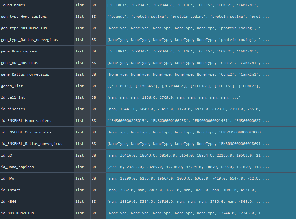
# There are two way of enrich data:
# * each data separately:

# Human protein Atlas data
enr.enriche_specificiti()

HPA = enr.get_HPA
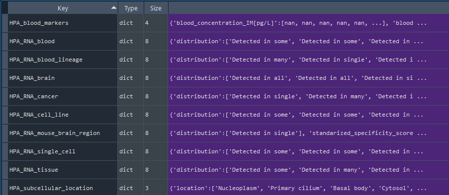
# KEGG data
enr.enriche_KEGG()

KEGG = enr.get_KEGG
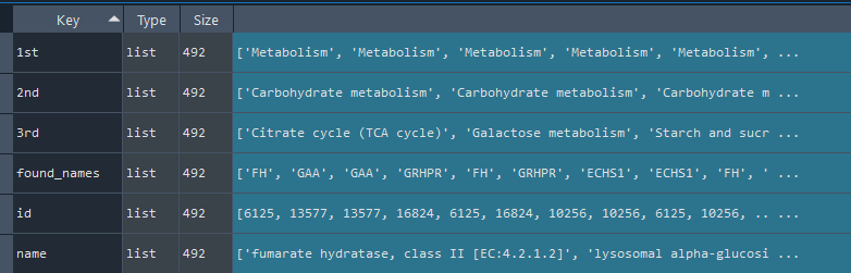
# GO-TERM data
enr.enriche_GOTERM()

GOTERM = enr.get_GO_TERM
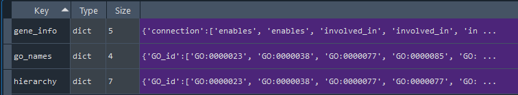
# Reactome data
enr.enriche_REACTOME()

REACTOME = enr.get_REACTOME
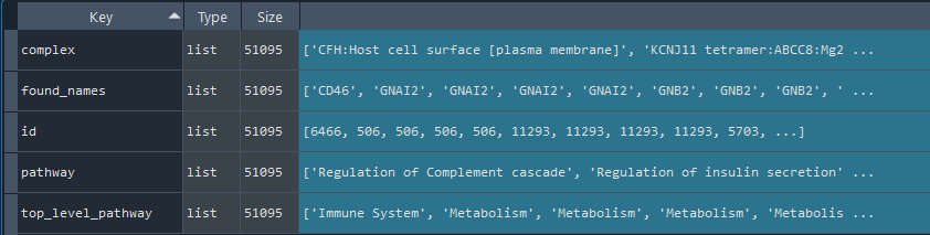
# Human Diseases data
enr.enriche_DISEASES()

DISEASES = enr.get_DISEASES
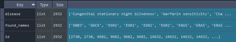
# ViMic data
enr.enriche_ViMIC()

ViMIC = enr.get_ViMIC
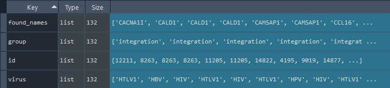
# IntAct data
enr.enriche_IntAct()

IntAct = enr.get_IntAct
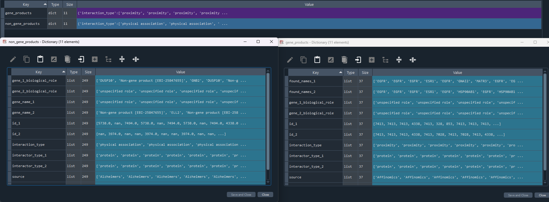
# STRING data
enr.enriche_STRING()

STRING = enr.get_STRING
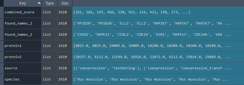
# CellCon data
enr.enriche_CellCon()

CellConnections = enr.get_CellCon
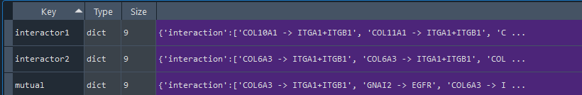
# RNAseq data
enr.enriche_RNA_SEQ()

RNASEQ = enr.get_RNA_SEQ
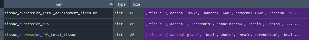
# * all data in parallel:


enr.full_enrichment()


# get_results can be used for return all data enriched separately like above ^^^
results = enr.get_results
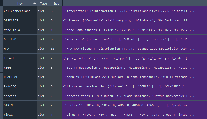
# import the Analysis class from the Enrichment module
from gedspy import Analysis

# create instance of the Analysis class with results from get_results
ans = Analysis(results)

# adjustment of analysis parameters
# for more details go to documentation on GitHub

# network parameters
ans.networks_metadata

# interactions parameters
ans.interactions_metadata

# set analysis parameter (default parameters check in documentation on GitHub)
ans.set_p_value(value = 0.05)
ans.set_test(test = 'FISH')
ans.set_correction(correction = None)

ans.networks_metadata
# Overrepresentation analysis
# There are two way of enrich data:
# * each data separately:

# GO-TERM
ans.GO_overrepresentation()

go = ans.get_GO_statistics
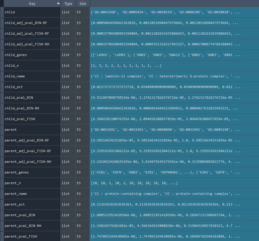
# KEGG
ans.KEGG_overrepresentation()

kegg = ans.get_KEGG_statistics
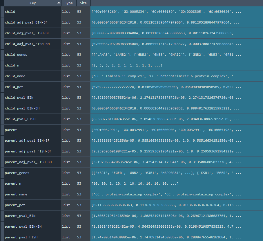
# Reactome
ans.REACTOME_overrepresentation()

reactome = ans.get_REACTOME_statistics
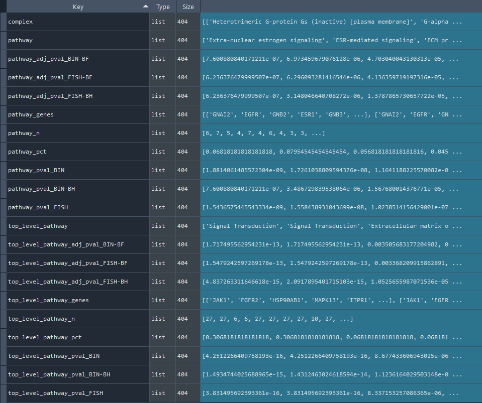
# ViMic
ans.ViMIC_overrepresentation()

vimic = ans.get_ViMIC_statistics
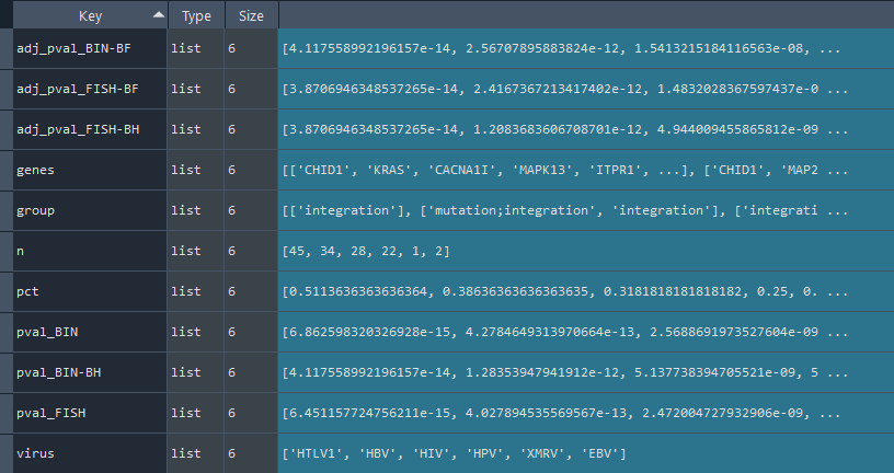
# Human diseases
ans.DISEASES_overrepresentation()

diseases = ans.get_DISEASE_statistics
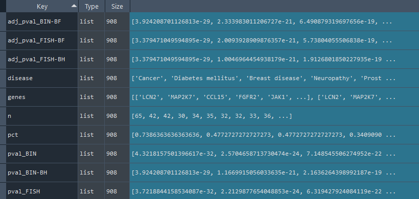
# Specificity (HPA)
ans.features_specificity()

spec = ans.get_specificity_statistics
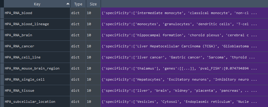
# Interactions (STRING/IntAct)
ans.gene_interaction()

inter = ans.get_features_interactions_statistics
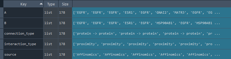
# Reactome paths network
ans.REACTOME_network()

reactome_net = ans.get_REACTOME_network
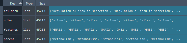
# KEGG paths network
ans.KEGG_network()

kegg_net = ans.get_KEGG_network
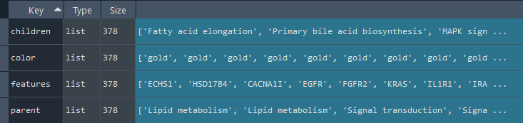
# GO-TERM terms network
ans.GO_network()

go_net = ans.get_GO_network
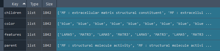
# * all data in parallel:


ans.full_analysis()


# get_results can be used for return all data enriched separately like above ^^^
results2 = ans.get_full_results
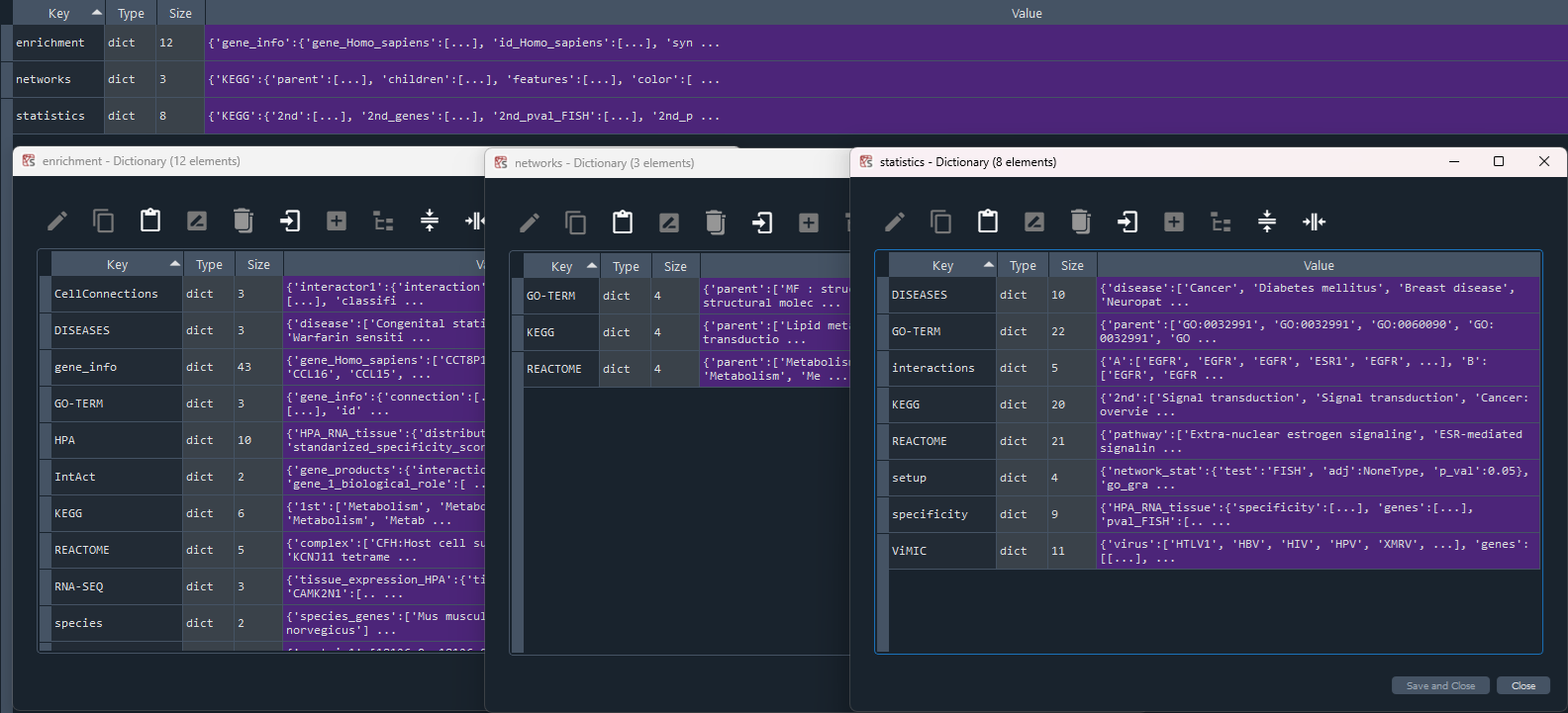
# import the Visualization class from the Enrichment module
from gedspy import Visualization

# load library JVG - display and adjustment Networks and Bar plots
from JVG import JVG

# create instance of the Visualization class with results from get_full_results
vis = Visualization(results2)
# gene type
plot  =  vis.gene_type_plot(cmap = 'summer', image_width = 6, image_high = 6, font_size = 15)

graph = JVG.MplEditor(plot)
graph.edit()
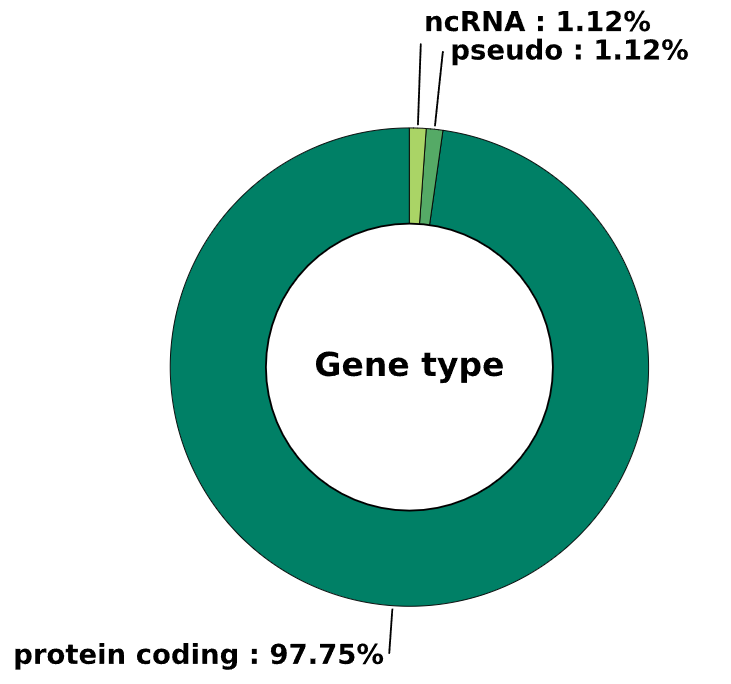
# GO-TERM
plot  =  vis.GO_plot(p_val = 0.05,
                    test = 'FISH',
                    adj = None,
                    n = 20,
                    side = 'left',
                    color = 'blue',
                    width = 10,
                    bar_width = 0.5,
                    stat = 'p_val')

graph = JVG.MplEditor(plot)
graph.edit()
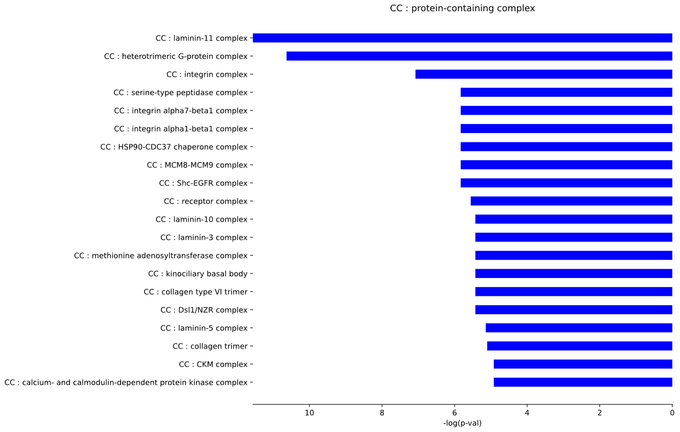
# Specificity (HPA)
plot  =  vis.SPECIFICITY_plot(p_val = 0.05,
                    test = 'FISH',
                    adj = None,
                    n = 25,
                    side = 'right',
                    color = 'bisque',
                    width = 10,
                    bar_width = 0.5,
                    stat = 'p_val')

graph = JVG.MplEditor(plot)
graph.edit()
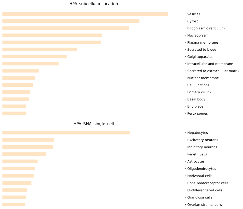
# KEGG
plot = vis.KEGG_plot(p_val = 0.05,
test = 'FISH',
adj = None,
n = 25,
side = 'right',
color = 'orange',
width = 10,
bar_width = 0.5,
stat = 'p_val')
graph = JVG.MplEditor(plot)
graph.edit()
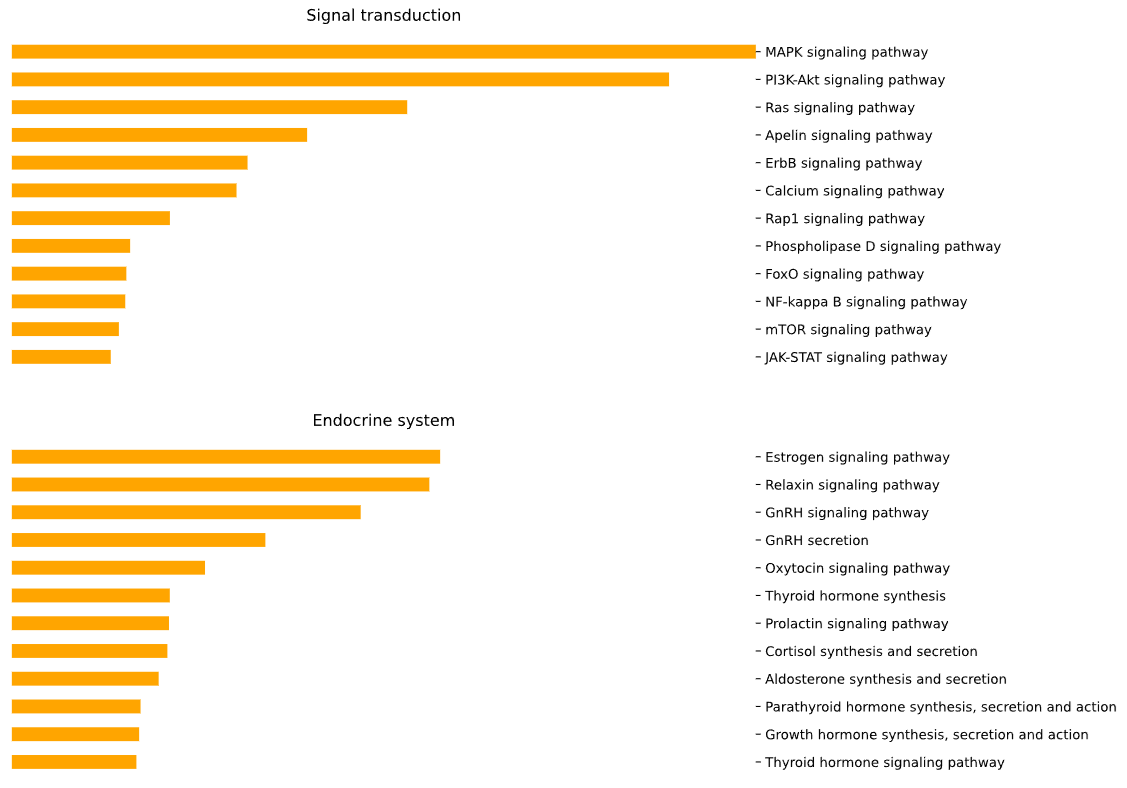
# Reactome
plot = vis.REACTOME_plot(p_val = 0.05,
test = 'FISH',
adj = None,
n = 25,
side = 'right',
color = 'silver',
width = 10,
bar_width = 0.5,
stat = 'p_val')
graph = JVG.MplEditor(plot)
graph.edit()
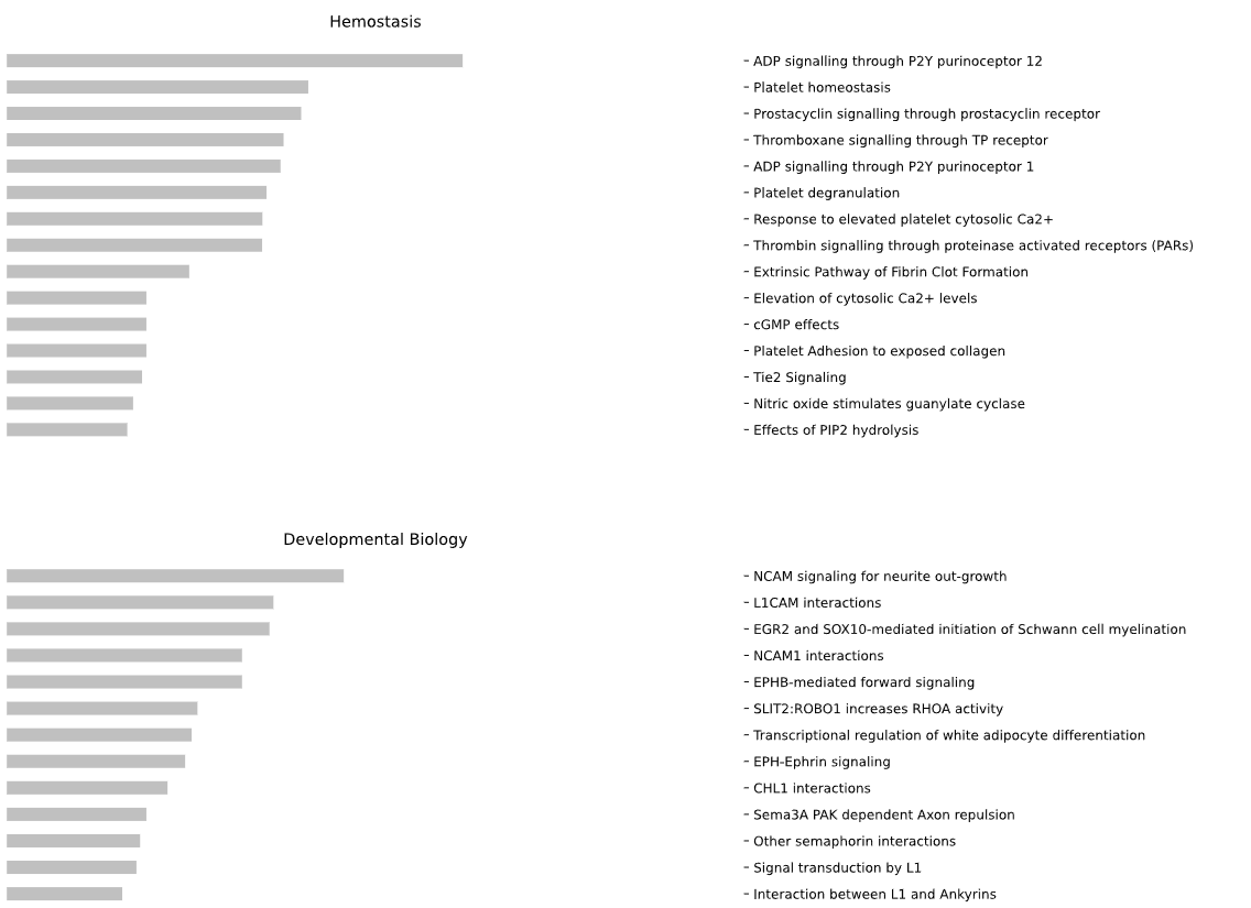
# Human diseases
plot = vis.DISEASES_plot(p_val = 0.05,
test = 'FISH',
adj = None,
n = 25,
side = 'right',
color = 'thistle',
width = 10,
bar_width = 0.5,
stat = 'p_val')
graph = JVG.MplEditor(plot)
graph.edit()
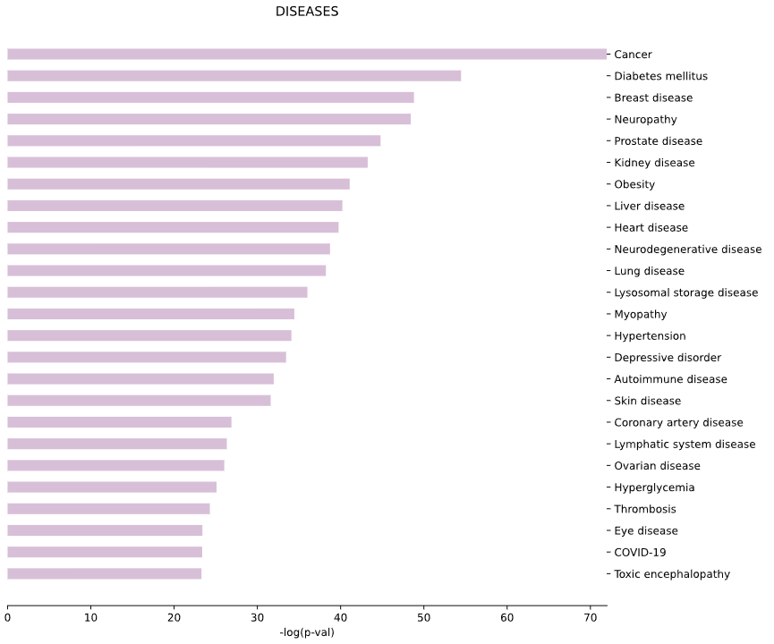
# ViMic
plot = vis.ViMIC_plot(p_val = 0.05,
test = 'FISH',
adj = None,
n = 25,
side = 'right',
color = 'aquamarine',
width = 10,
bar_width = 0.5,
stat = 'p_val')
graph = JVG.MplEditor(plot)
graph.edit()
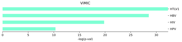
# blood markers
plot = vis.blod_markers_plot()
graph = JVG.MplEditor(plot)
graph.edit()
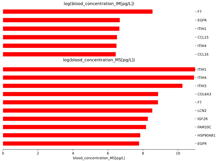
# GO-TERM network
go = vis.GOPa_network_create(
data_set = 'GO-TERM',
genes_inc = 10,
gene_int = True,
genes_only = True,
min_con = 2,
children_con = True,
include_childrend = True,
selected_parents = [],
selected_genes = [])
nt = JVG.NxEditor(go)
nt.edit()
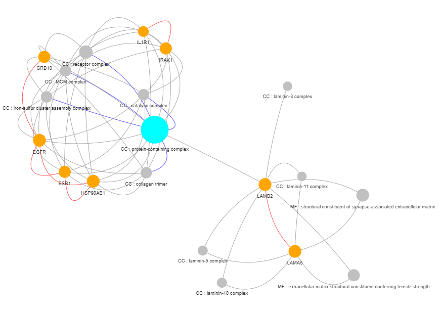
# KEGG network
kegg = vis.GOPa_network_create(
data_set = 'KEGG',
genes_inc = 10,
gene_int = True,
genes_only = True,
min_con = 2,
children_con = True,
include_childrend = True,
selected_parents = ['Nervous system', 'Cell motility'],
selected_genes = [])
nt = JVG.NxEditor(kegg)
nt.edit()
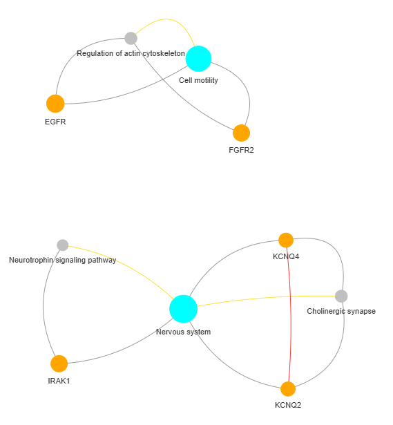
# Reactome network
react = vis.GOPa_network_create(
data_set = 'REACTOME',
genes_inc = 10,
gene_int = True,
genes_only = True,
min_con = 2,
children_con = False,
include_childrend = False,
selected_parents = [],
selected_genes = ['F7', 'LAMA5'])
nt = JVG.NxEditor(react)
nt.edit()
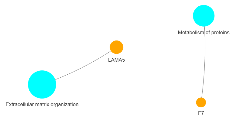
# Gene interactions network
inter = vis.GI_network_create()
nt = JVG.NxEditor(inter)
nt.edit()
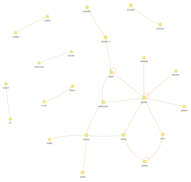
# AUTO-ML
ml = vis.AUTO_ML_network(
genes_inc = 10,
gene_int = True,
genes_only = True,
min_con = 1,
children_con = True,
include_childrend = True,
selected_parents = ['Cell motility', 'Development and regeneration'],
selected_genes = ['JAK1', 'KRAS'])
nt = JVG.NxEditor(ml)
nt.edit()
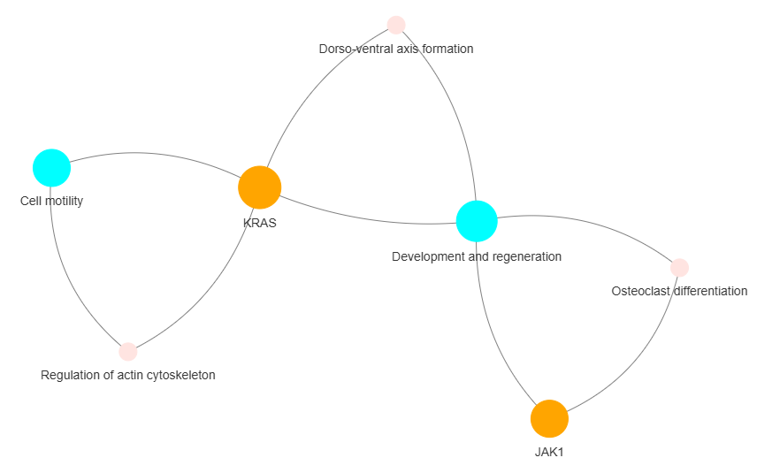
# RNAseq
seq = vis.gene_scatter(
colors = 'viridis',
species = 'human',
hclust = 'complete',
img_width = None,
img_high = None,
label_size = None,
x_lab = 'Genes',
legend_lab = 'log(TPM + 1)')
graph1 = JVG.MplEditor(seq['tissue_expression_HPA'])
graph1.edit()
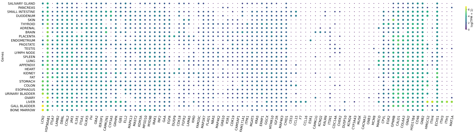
graph2 = JVG.MplEditor(seq['tissue_expression_RNA_total_tissue'])
graph2.edit()
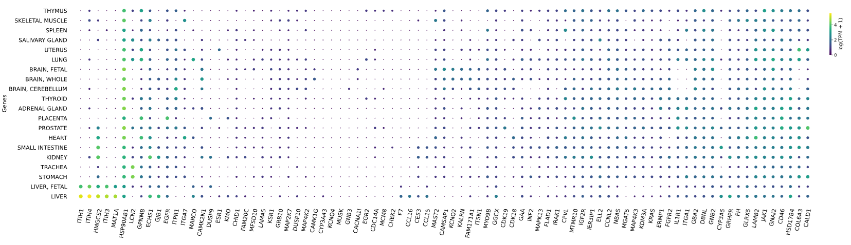
graph3 = JVG.MplEditor(seq['tissue_expression_fetal_development_circular'])
graph3.edit()
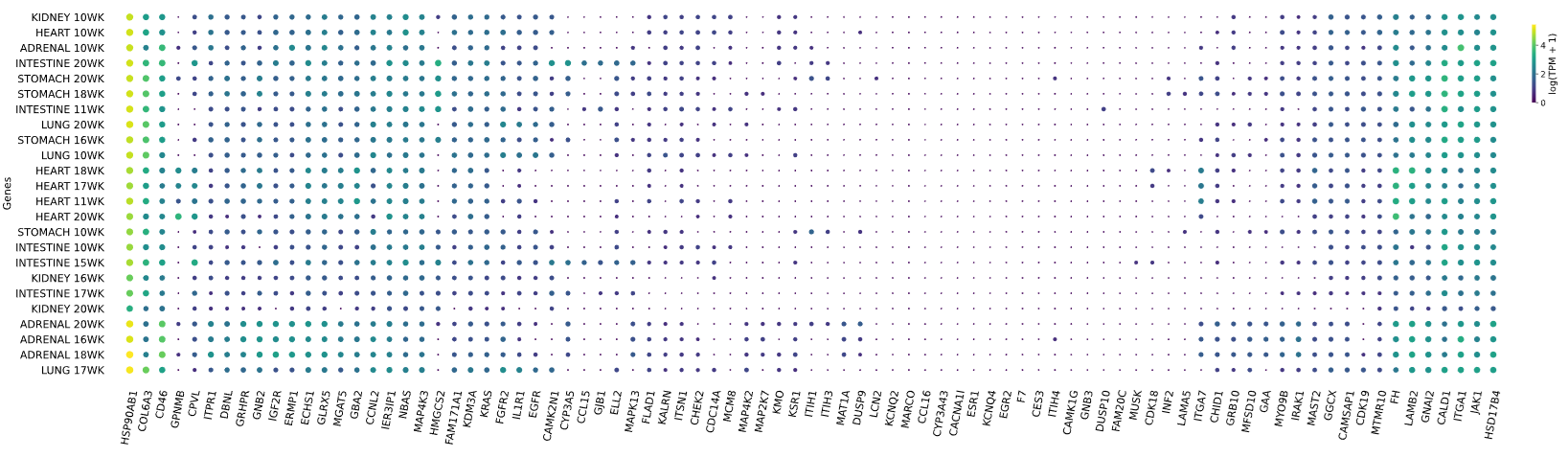
11. Example enrichment analysis of double sets
# Example analysis gene lists
gene_list = ['CACNA1I','CALD1','CAMK1G','CAMK2N1','CAMSAP1','CCL15','CCL16','CCNL2','CCT8P1','CD46','CDC14A','CDK18','CDK19','CES3','CHEK2',
'CHID1','COL6A3','CPVL','CYP3A43','CYP3A5','DBNL','DUSP10','DUSP9','ECHS1','EGFR','EGR2','ELL2','ERMP1','ESR1','F7','FAM171A1',
'FAM20C','FGFR2','FH','FLAD1','FUT3','GAA','GBA2','GGCX','GJB1','GLRX5','GNAI2','GNB2','GNB3','GPNMB','GRB10','GRHPR','HMGCS2',
'HSD17B4','HSP90AB1','IER3IP1','IGF2R','IL1R1','INF2','IRAK1','ITGA1','ITGA7','ITIH1','ITIH3','ITIH4','ITPR1','ITSN1','JAK1',
'KALRN','KCNQ2','KCNQ4','KDM3A','KMO','KRAS','KSR1','LAMA5','LAMB2','LCN2','MAP2K7','MAP4K2','MAP4K3',
'MAPK13','MARCO','MAST2','MAT1A','MATR3','MCM8','MFSD10','MGAT5','MTMR10','MUSK','MYO9B','NBAS']
gene_list2 = ['NCOA6','NCSTN','NDUFA4','NEK4', 'UDT2','NUP210','ORC3L','PAOX','PEMT','PEX14','PFKL','PHKA2','PIM1','PLXND1','PMM1','PON3','POR','PPARG','PPARGC1B',
'PRKCE','PTK2B','PTP4A1','PTPN23','PTPRF','PTPRK','RARA','RNF10','RNF14','RNF165','ROCK2','RRBP1','RREB1','SCN1A','SDC1','SERPINA1','SERPINA10','SFXN5',
'SHROOM1','SIL1','SIRPA','SLC12A7','SLC13A3','SLC16A2','SLC17A7','SLC22A23','SLC22A9','SLC25A11','SLC25A25','SLC38A3','SLC45A3','SLC4A5','SLC5A1','SLC7A2',
'SLC8A3','SLC9A6','SLCO1A2','SLCO1B3','SMARCA2','NX4','SORBS1','SPEN','SPR','SRF','STAB1','STAT1','SUCLG2','SULT1B1','SULT1E1','TBC1D2B','TCHP','TGFBI',
'TGOLN2','THPO', 'IMM13','TLK2','TMEM62','TNFSF14','TNK2','TNS1','TPI1','TRIB3','TRMT11','TTYH3']
# import the Enrichment & Analysis classes from the Enrichment module
from gedspy import Enrichment
from gedspy import Analysis
#SET1
# create instance of the Enrichment class
enr = Enrichment()
# select featrues from genes/proteins list for Homo sapiens / Mus musculus / Rattus norvegicus for first gene_list
enr.select_features(gene_list)
# conduct full enrichment
enr.full_enrichment()
# get results for first set
results1 = enr.get_results
# create instance of the Analysis class
ans = Analysis(results1)
# set parameters or leave default - see manual on GitHub
ans.set_p_value(value = 0.05)
ans.set_test(test = 'FISH')
ans.set_correction(correction = None)
# ! parameters for both analyses (set1 and set2) must be the same !
# conduct full analyses
ans.full_analysis()
# get full results for first set
results1 = ans.get_full_results
# create instance of the Enrichment class
enr = Enrichment()
# select featrues from genes/proteins list for Homo sapiens / Mus musculus / Rattus norvegicus for second gene_list
enr.select_features(gene_list2)
# conduct full enrichment
enr.full_enrichment()
# get results for second set
results2 = enr.get_results
# create instance of the Analysis class
ans = Analysis(results2)
# set parameters or leave default - see manual on GitHub
ans.set_p_value(value = 0.05)
ans.set_test(test = 'FISH')
ans.set_correction(correction = None)
# ! parameters for both analyses (set1 and set2) must be the same !
# conduct full analyses
ans.full_analysis()
# get full results for second set
results2 = ans.get_full_results
# import the DSA class from the Enrichment module
from gedspy import DSA
# create instance of the DSA class with results from get_full_results for set1 and set2
dsa_compare = DSA(results1, results2)
# DSA analysis
# There are two way of enrich data:
# * each data separately:
# GO-TERM DSA
dsa_compare.GO_diff()
go = dsa_compare.get_GO_diff
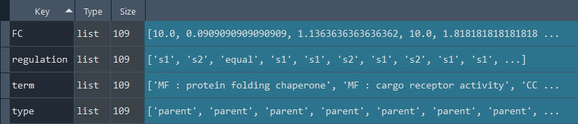
# KEGG DSA
dsa_compare.KEGG_diff()
kegg = dsa_compare.get_KEGG_diff

# Reactome DSA
dsa_compare.REACTOME_diff()
reactome = dsa_compare.get_REACTOME_diff
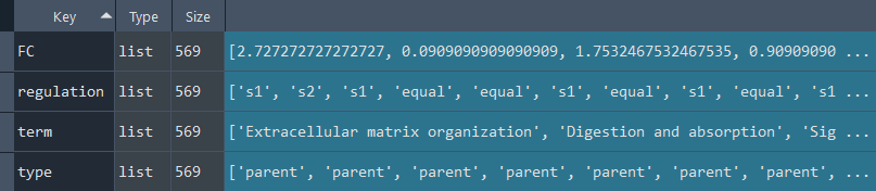
# Specificity (HPA) DSA
dsa_compare.spec_diff()
hpa = dsa_compare.get_specificity_diff
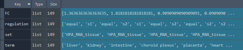
# Gene interactions DSA
dsa_compare.gi_diff()
GI = dsa_compare.get_GI_diff
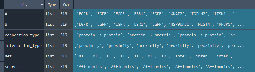
# Networks DSA
dsa_compare.network_diff()
networks = dsa_compare.get_networks_diff
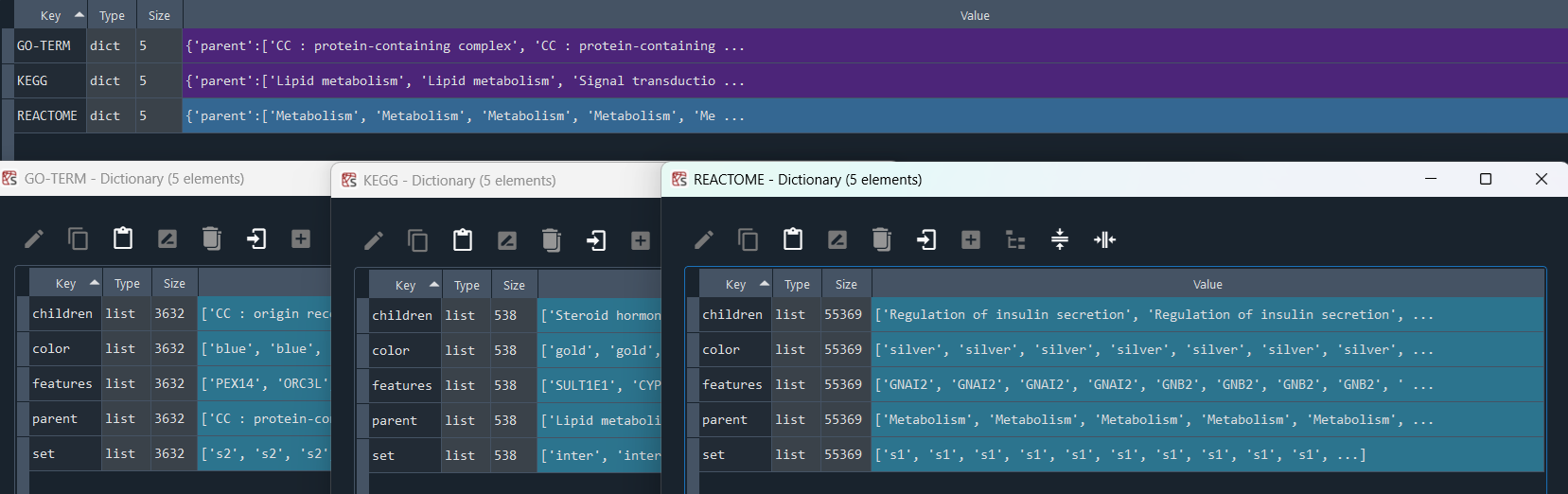
# Inter Terms DSA
dsa_compare.inter_processes()
inter_terms = dsa_compare.get_inter_terms
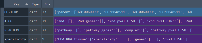
# Connections DSA
dsa_compare.connections_diff()
connections = dsa_compare.get_set_to_set_con
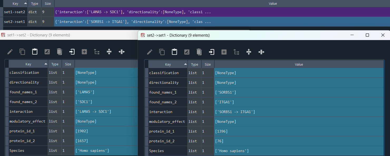
# * all data in parallel:
dsa_compare.full_analysis()
# get_results can be used for return all DSA data like above ^^^
results3 = dsa_compare.get_results
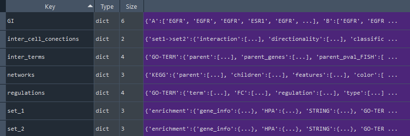
# import the VisualizationDES class from the Enrichment module
from gedspy import VisualizationDES
# load library JVG - display and adjustment Networks and Bar plots
from JVG import JVG
# create instance of the VisualizationDES class with results from get_results for set1 and set2 DSA results
vis_des = VisualizationDES(results3)
# Gene type
plot = vis_des.diff_gene_type_plot(
set1_name = 'Set 1',
set2_name = 'Set 2',
image_width = 12,
image_high = 6,
font_size = 15)
graph = JVG.MplEditor(plot)
graph.edit()
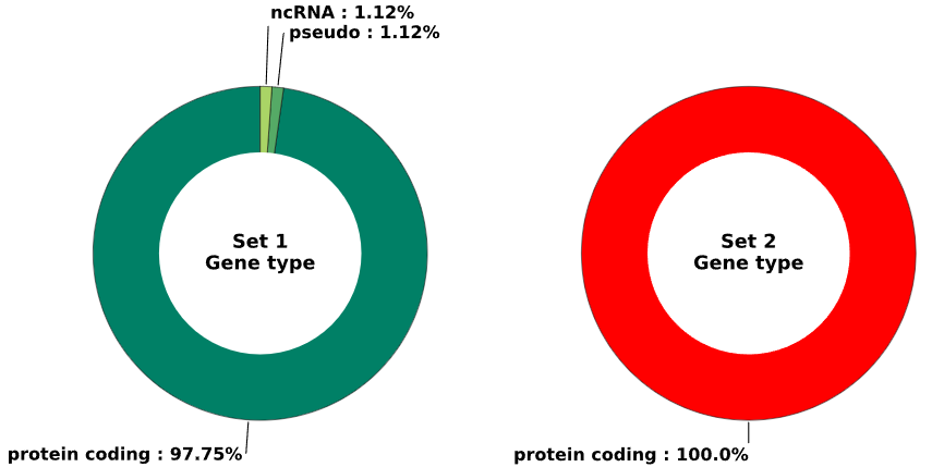
# GO-TERM
plot = vis_des.diff_GO_plot(
p_val = 0.05,
test = 'FISH',
adj = 'BH',
n = 25,
min_terms = 5,
selected_parent = [],
width = 10,
bar_width = 0.5,
stat = 'p_val',
sep_factor = 50)
graph = JVG.MplEditor(plot)
graph.edit()
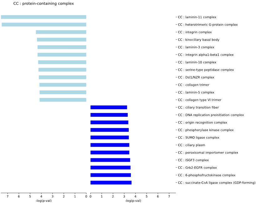
# KEGG
plot = vis_des.diff_KEGG_plot(
p_val = 0.05,
test = 'FISH',
adj = 'BH',
n = 25,
min_terms = 2,
selected_parent = [],
width = 10,
bar_width = 0.5,
stat = 'p_val',
sep_factor = 50)
graph = JVG.MplEditor(plot)
graph.edit()
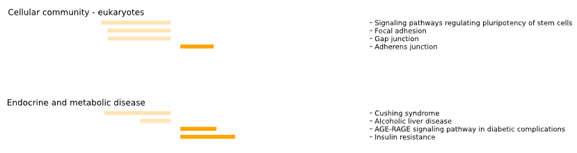
# Reactome
plot = vis_des.diff_REACTOME_plot(
p_val = 0.05,
test = 'FISH',
adj = 'BH',
n = 25,
min_terms = 5,
selected_parent = [],
width = 10,
bar_width = 0.5,
stat = 'n',
sep_factor = 50)
graph = JVG.MplEditor(plot)
graph.edit()
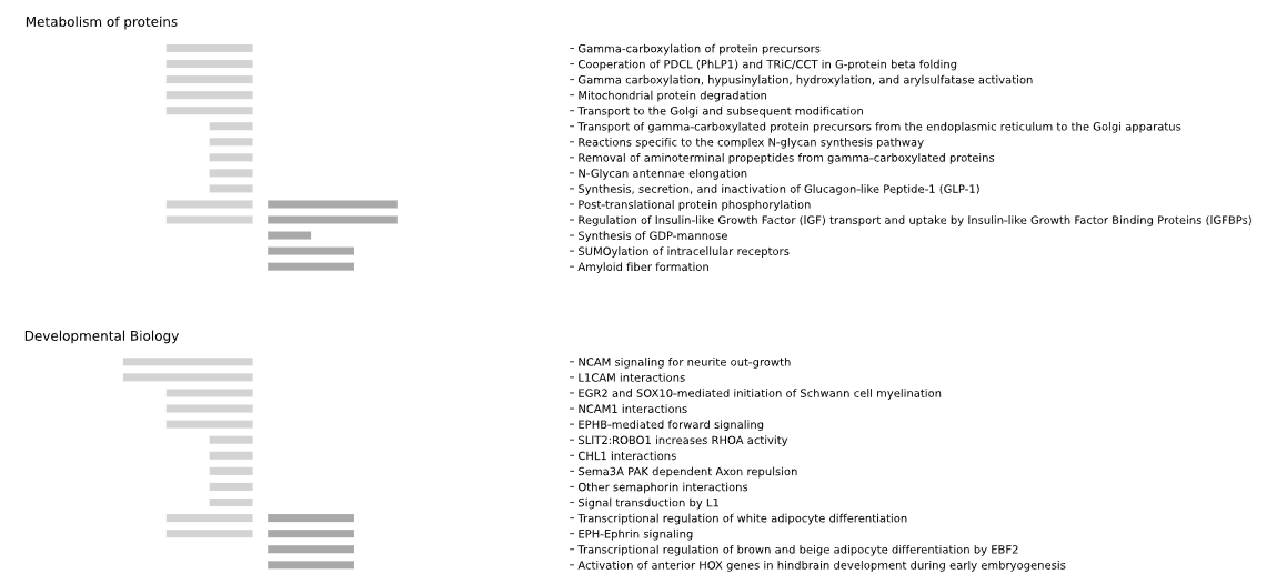
# Specificity (HPA)
plot = vis_des.diff_SPECIFICITY_plot(
p_val = 0.05,
test = 'FISH',
adj = 'BH',
n = 6,
min_terms = 1,
selected_set = [],
width = 10,
bar_width = 0.5,
stat = 'p_val',
sep_factor = 15)
graph = JVG.MplEditor(plot)
graph.edit()
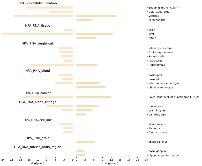
# GO-TERM network
go = vis_des.diff_GOPa_network_create(data_set = 'GO-TERM',
genes_inc = 10,
gene_int = True,
genes_only = True,
min_con = 2,
children_con = False,
include_childrend = True,
selected_parents = [],
selected_genes = [])
nt = JVG.NxEditor(go)
nt.edit()
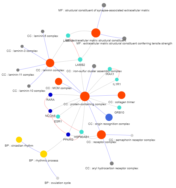
# KEGG network
kegg = vis_des.diff_GOPa_network_create(data_set = 'KEGG',
genes_inc = 10,
gene_int = True,
genes_only = True,
min_con = 2,
children_con = False,
include_childrend = True,
selected_parents = [],
selected_genes = [])
nt = JVG.NxEditor(kegg)
nt.edit()
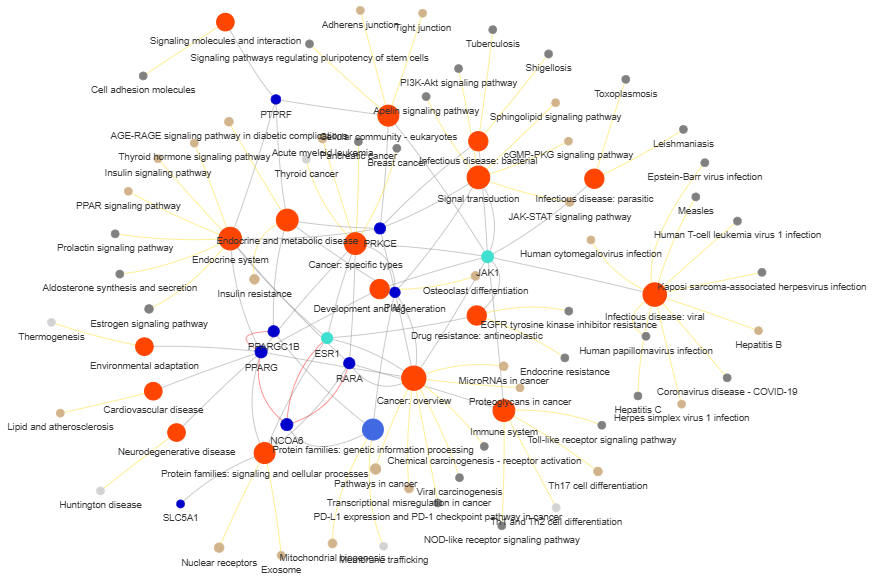
# Reactome network
reactome = vis_des.diff_GOPa_network_create(data_set = 'REACTOME',
genes_inc = 10,
gene_int = True,
genes_only = True,
min_con = 2,
children_con = False,
include_childrend = True,
selected_parents = [],
selected_genes = [])
nt = JVG.NxEditor(reactome)
nt.edit()
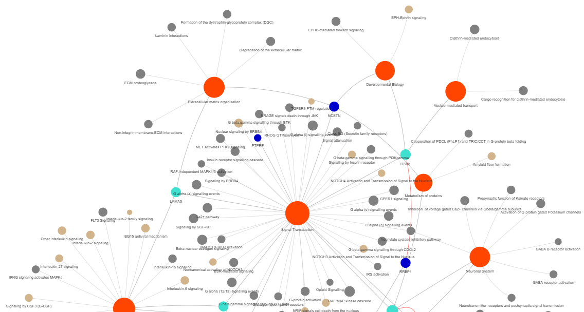
# GI network
gi = vis_des.diff_GI_network_create(min_con = 2)
nt = JVG.NxEditor(gi)
nt.edit()
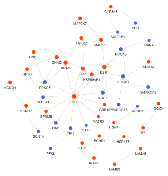
# AMUTO-ML network
ml = vis_des.diff_AUTO_ML_network(
genes_inc = 10,
gene_int = True,
genes_only = True,
min_con = 2,
children_con = False,
include_childrend = False,
selected_parents = [],
selected_genes = [])
nt = JVG.NxEditor(ml)
nt.edit()
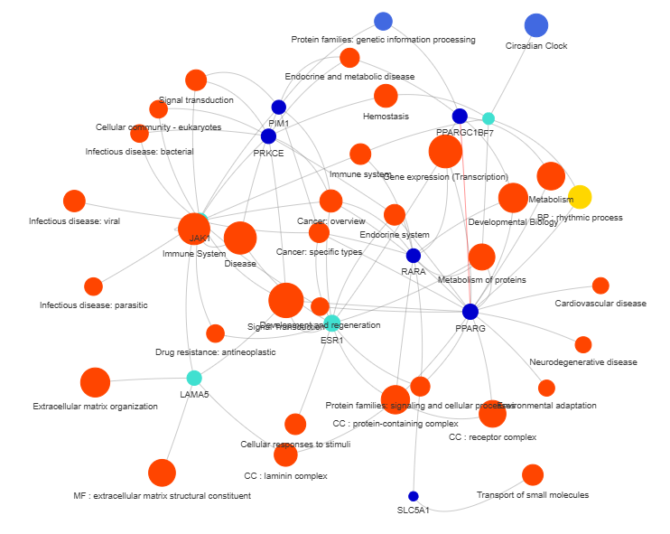
# RNAseq
seq = vis_des.diff_gene_scatter(
set_num = 2,
colors = 'viridis',
species = 'human',
hclust = 'complete',
img_width = None,
img_high = None,
label_size = None,
x_lab = 'Genes',
legend_lab = 'log(TPM + 1)',
selected_list = [])
graph1 = JVG.MplEditor(seq['tissue_expression_HPA'])
graph1.edit()
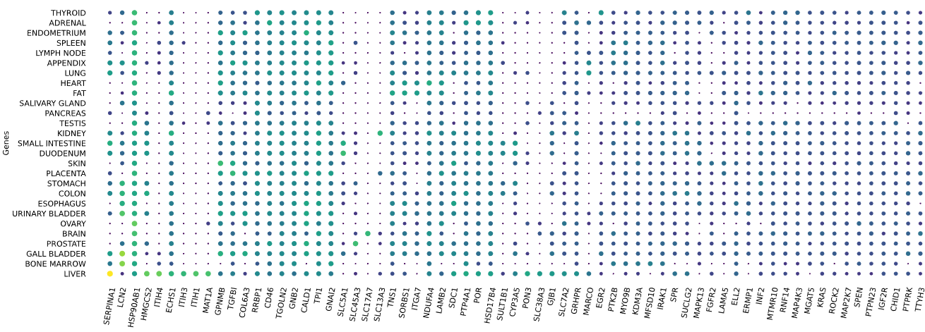
graph2 = JVG.MplEditor(seq['tissue_expression_RNA_total_tissue'])
graph2.edit()
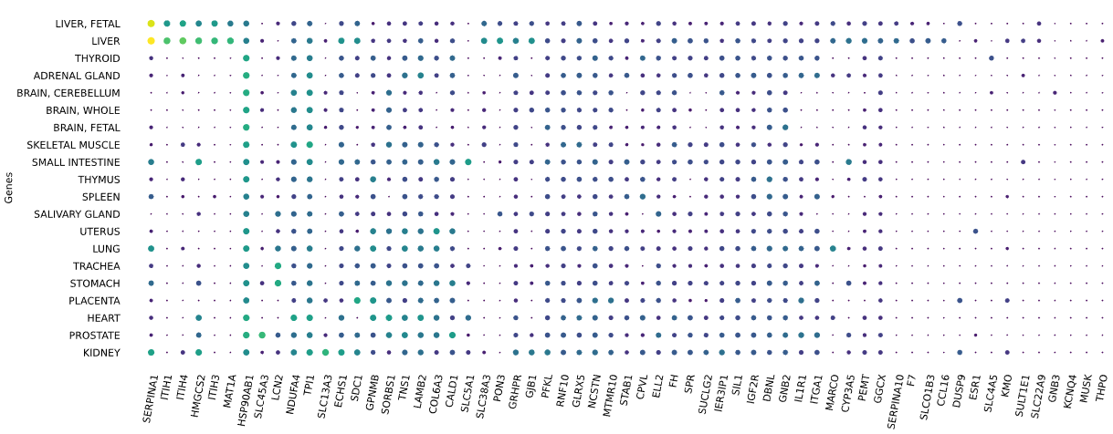
graph3 = JVG.MplEditor(seq['tissue_expression_fetal_development_circular'])
graph3.edit()
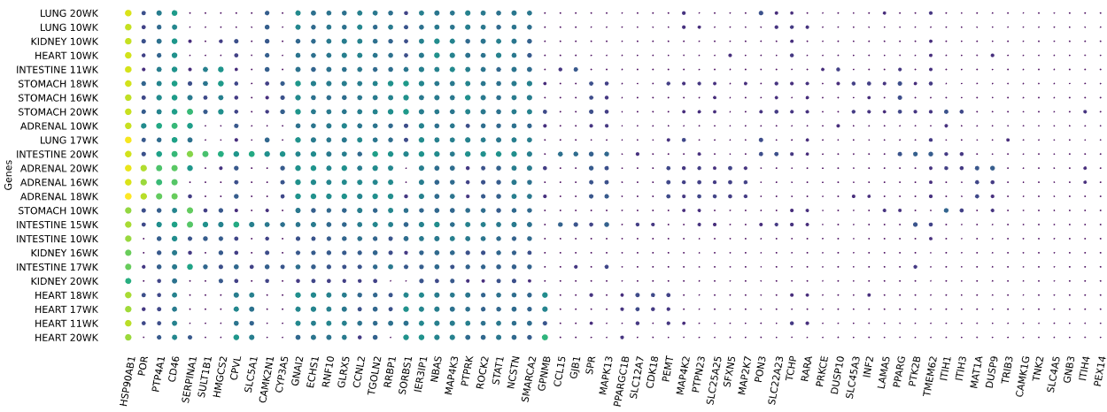
Heatmap - adjusted data
Get data - example:
data = dsa_compare.get_full_GO()
# Adjust terms in the data (optional)
term_col = 'child_name'
set_col = 'set'
sets = {'s1':'down','s2':'up'}
title= 'BP : developmental process'
fig_size = (8,15)
figure = enrichment_heatmap(data = data,
stat_col = stat_col,
term_col = term_col,
set_col = set_col,
sets = sets,
title = title,
fig_size = fig_size,
font_size = 16,
scale = True)
figure.savefig(
"heatmap.svg",
format="svg",
dpi=300,
bbox_inches="tight"
)

Have fun JBS©
Release history Release notifications | RSS feed


Download files
Download the file for your platform. If you're not sure which to choose, learn more about installing packages.
Source Distribution
Built Distribution
Filter files by name, interpreter, ABI, and platform.
If you're not sure about the file name format, learn more about wheel file names.
Copy a direct link to the current filters
File details
Details for the file gedspy-2.2.0.tar.gz.
File metadata
- Download URL: gedspy-2.2.0.tar.gz
- Upload date:
- Size: 129.6 kB
- Tags: Source
- Uploaded using Trusted Publishing? No
- Uploaded via: twine/6.2.0 CPython/3.11.9
File hashes
| Algorithm | Hash digest | |
|---|---|---|
| SHA256 |
089e1a300b5fd0256d2ddcfc56ef2d145cc351d4369cf9ad799f2ddf18b71caf
|
|
| MD5 |
d954f2a4113e24093ce2ba29ca26aa2f
|
|
| BLAKE2b-256 |
fa4cf4e864436885b9fcbdbeee1140870d8d1158276627fbc99158e93a76b947
|
File details
Details for the file gedspy-2.2.0-py3-none-any.whl.
File metadata
- Download URL: gedspy-2.2.0-py3-none-any.whl
- Upload date:
- Size: 111.3 kB
- Tags: Python 3
- Uploaded using Trusted Publishing? No
- Uploaded via: twine/6.2.0 CPython/3.11.9
File hashes
| Algorithm | Hash digest | |
|---|---|---|
| SHA256 |
a56f372fe44dde6756520c71daee37c517624e97a628518f3321d223a1de710d
|
|
| MD5 |
ca4d1eb28c816ee29ec8da3af66d4b7c
|
|
| BLAKE2b-256 |
680de0e4d4557370177fc40413d8fcda91540ab215fb266f3e0b993e8915a263
|


