
gee-biophys
Custom temporal exports of biophysical variable retrievals (LAIe, FAPAR, FCOVER) from Sentinel-2 imagery.
This tool enables users to define custom time windows, temporal frequency, regions, and export settings for Sentinel-2–based biophysical variable retrievals using a simple YAML configuration file. It provides both:
- a Python API, and
- a Command-Line Interface (CLI):
gee-biophys.
Overview
gee-biophys enables flexible and reproducible export of time-series vegetation biophysical maps, addressing the need for user-defined temporal aggregation of Sentinel-2–derived biophysical variable retrievals.
The tool builds on the PROSAIL-based s2biophys retrieval framework, and also supports a local-only Grounded EO Gaussian-process model trained directly on in situ validation data. Together, the package supports consistent estimates of:
- Effective Leaf Area Index (LAIe)
- Fraction of Absorbed Photosynthetically Active Radiation (FAPAR)
- Fractional Vegetation Cover (FCOVER)
- Local-only Grounded EO predictions for LAI and FAPAR
Each export includes:
mean— aggregated trait valuestdDev— within-period variabilitycount— number of valid observations
Features
- Flexible temporal definitions: fixed (e.g. monthly, quarterly) or custom seasonal windows
- Spatial inputs via bounding box, GeoJSON geometry, or a square defined in metres
- Modular YAML configuration for reproducibility
- Exports directly to Google Earth Engine assets, Google Drive, or Google Cloud Storage
- Available as both a Python package and CLI tool
- Supports three model families: s2biophys, SL2P, and a local-only Grounded EO Gaussian-process model
- Grounded EO is available for LAI and FAPAR only and requires the xee-local export mode
Installation
Using pip
Create a clean virtual environment (e.g. using conda or venv). Recommended Python version 3.12:
conda create -n [ENV_NAME] python=3.12
conda activate [ENV_NAME]
pip install gee-biophys
Alternative installation — Install from source
conda create -n [ENV_NAME] python=3.12
conda activate [ENV_NAME]

git clone https://github.com/speckerf/gee_biophys.git
cd gee_biophys

pip install -e .
Usage
Start Exports
1. Command-line interface
gee-biophys --config path_to_yaml.yaml (--public)
- The
--config(or-c) argument is required and must point to a valid YAML configuration file. - The
--publicargument is optional and can be specified if the createImageCollectionshould be public to all GEE-users.
2. Python interface
from gee_biophys.cli import run_pipeline

run_pipeline(config='path_to_yaml.yaml')
Wait for exports to finish:
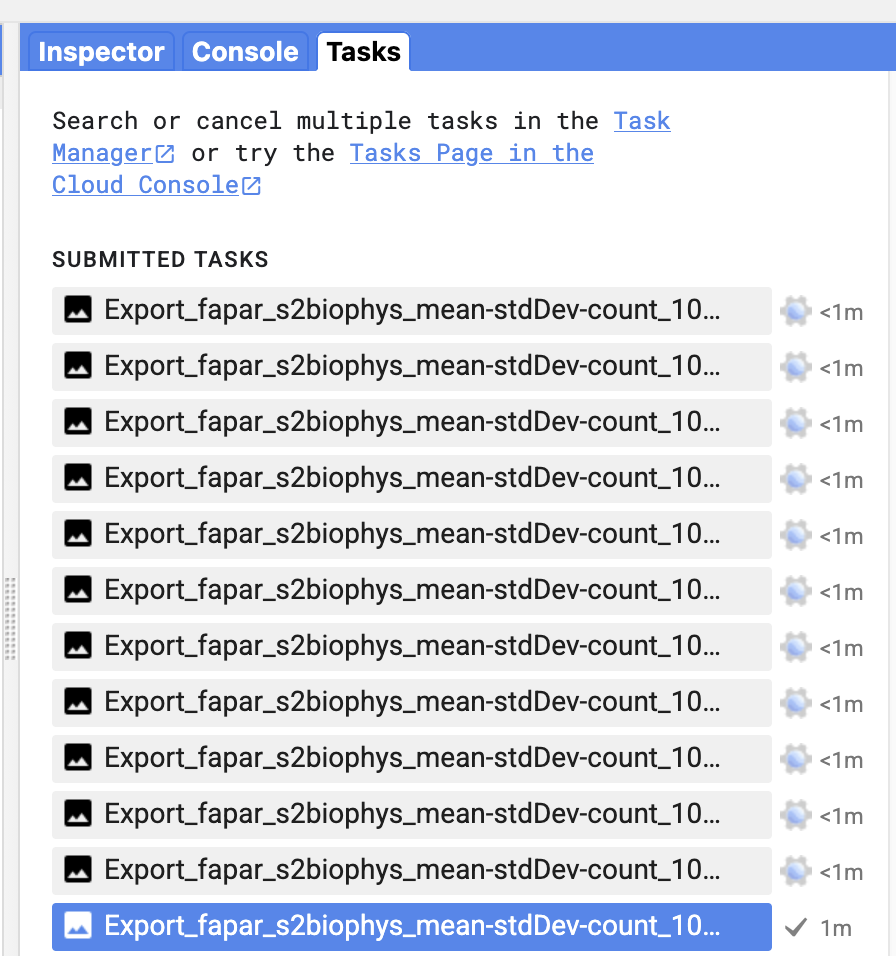
The tool will start an Earth Engine export task for each exported time period. So the temporal frequency and the total time window determine the number of export tasks to execute.
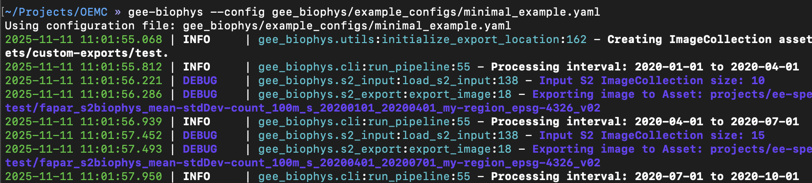
Check the progress of the exports in the code editor directly:
Alternatively, check progress directly using the logged task ID: earthengine task info [TASK_ID]
Visualize results
To visualize results, please use the following earth-engine app: here. Note that this requires that the option --public was set when running gee-biophys.
Alternatively, the source code of the app can also be directly to visualize a non-public ImageCollection.
Example Configuration
Example configuration files are provided in https://github.com/speckerf/gee_biophys/tree/main/example_configs.
Minimal Example Config
# ============     GEE-Biophys  ================
# Minimal Example (small exports for testing)
# ==============================================

spatial:
  type: bbox
  bbox: [7.1, 46.1, 7.2, 46.2]
  region_name: my-region

temporal:
  start: "2020-01-01"
  end:   "2023-01-01"
  cadence:
    type: fixed
    interval: quarterly

variables:
  model: s2biophys
  variable: fapar

export:
  destination: asset
  collection_path: "projects/ee-speckerfelix/assets/custom-exports/test" # CHANGE
  project_id: "ee-speckerfelix" # CHANGE
  crs: "EPSG:4326" # EPSG code or LOCAL_UTM (automatic)
  scale: 100
  max_pixels: 100_000_000_000

options:
  max_cloud_cover: 50
  csplus_band: cs
  cs_plus_threshold: 0.70
  clip_min_max: true # if true, clips predictions to (0, 1) for fapar and fcover, and (0, 8) for laie/lai

version: "v02"
Square regions
spatial:
  type: square
  square_center: [8.4, 47.48]  # longitude, latitude
  square_length: 2000         # side length in metres
The square is centred and aligned in local UTM, then transformed to longitude/latitude. Its size is independent of export.crs, including EPSG:4326. Use this pair instead of bbox or geojson_path; the centre must be within UTM latitudes (80°S–84°N).
Biome/land-cover-specific s2biophys
Choose a named, independently optimized three-member ensemble for GEE or xee-local:
variables:
  model: s2biophys-biome-lc-specific
  biome_lc_name: temperate_broadleaf_forest
  variable: fapar  # laie, fapar, or fcover
Names: cold_evergreen_forest, open_tundra, arid_shrubland, temperate_nonforest, temperate_broadleaf_forest, temperate_evergreen_forest, tropical_forest, mediterranean_forest. Numeric selectors are not accepted. The selected ensemble predicts the full scene, without masking to its vegetation class; normal input/cloud masks still apply (and the GEE path retains its water mask). Uncertainty currently reuses the global calibration table.
Small examples: broadleaf / GEE, shrubland / GEE, nonforest / xee-local. Compare both models in the executed notebook.
Grounded EO local-only configuration
The Grounded EO model is a local, in situ–trained Gaussian-process predictor. It is currently supported only for the variables lai and fapar, and it requires the xee-local export destination because prediction runs locally on the exported xarray dataset.
variables:
  model: groundedeo
  variable: lai

export:
  destination: xee-local
  folder: "/path/to/local/export"
  crs: "EPSG:4326"
  scale: 100
This model returns local outputs with the naming convention:
grounded_lai_mean,grounded_lai_stdgrounded_fapar_mean,grounded_fapar_std
External notebook entrypoint (stack/composite + model comparison)
You can use gee_biophys directly from an external Jupyter notebook to:
-
load Sentinel-2 data for one interval as full stack or as one composite,
-
fetch it locally as an xarray dataset via xee,
-
run one or multiple models for map-to-map comparison.
-
see notebooks/
Reference Template
A fully commented reference configuration file is available here. A minimal example can be found here. Please check some example configuration files available here.
Configuration Structure
| Section | Purpose | Example |
|---|---|---|
spatial |
Defines the area of interest (bbox or GeoJSON) | [minLon, minLat, maxLon, maxLat] |
temporal |
Sets start/end dates and cadence (fixed or seasonal) | quarterly, monthly, yearly |
variables |
Selects the biophysical variable and retrieval model | fapar, laie, fcover |
export |
Configures export target and GEE project, CRS, spatial resolution, etc. | e.g. projects/ee-user/assets/... |
options |
Controls cloud masking and thresholds | max cloud cover, CS+ threshold |
version |
Records model version for reproducibility | "v02" |
Note: If you want to find a good balance between strict cloud masking and having enough cloud-free pixels for analysis, you can use the following script to explore and tune the three key parameters—CloudScore+ band, CloudScore+ threshold, and maximum CLOUDY_PIXEL_PERCENTAGE from the Sentinel-2 metadata: https://code.earthengine.google.com/716bee247685008f34b49c63d32b8447
File Naming Convention
Each exported asset or file follows a standardized and descriptive naming scheme generated automatically from the configuration parameters. The convention ensures reproducibility, traceability, and easy identification of spatial, temporal, and model settings.
The filename (or system:index in GEE) is constructed as:
{variable}_{model}_{bands}_{scale}m_s_{start}_{end}_{region-name}_{crs}_{version}
Example
fapar_s2biophys_mean-stdDev-count_100m_s_20200101_20201231_my-region_epsg-4326_v02
Note that exports with the same system:index will fail when writing to Earth Engine assets, as each asset ID must be unique, whereas they will overwrite existing files when exporting to Google Drive or Google Cloud Storage.
Citation
If you use gee-biophys in your research, please cite the associated publication (forthcoming):
Felix Specker, Anna K. Schweiger, Jean-Baptiste Féret et al. Advancing Ecosystem Monitoring with Global High-Resolution Maps of Vegetation Biophysical Properties, 29 September 2026, PREPRINT (Version 3) available at Research Square [https://doi.org/10.21203/rs.3.rs-6343364/v3]
Acknowledgments
The Open-Earth-Monitor Cyberinfrastructure (OEMC) project has received funding from the European Union’s Horizon Europe research and innovation programme under grant agreement No. 101059548.
1 maintainer

Metadata
1 maintainer
Release files for gee-biophys 2.1.3
For a detailed explanation of source distributions (sdists) and built distributions (wheels), please see the package formats documentation.
Source distribution (sdist)
| File | Size | Uploaded | |
|---|---|---|---|
| gee_biophys-2.1.3.tar.gz | 3.8 MB | Details |
Built distribution (wheel)
| File | Interpreter | ABI | Platform | Reset |
|---|---|---|---|---|
| gee_biophys-2.1.3-py3-none-any.whl | Python 3 | none | any | Details |
Total release size: 7.8 MB
Release files / gee_biophys-2.1.3.tar.gz
| Download URL | gee_biophys-2.1.3.tar.gz |
|---|---|
| Size | 3.8 MB |
| Tags | Source |
|
SHA-256 checksum How to use checksums |
fc3ddea4cf8e85ae0aa421dab7a16bb206010406bfb1e1e5faaa756165585d03
|
|
BLAKE2b-256 checksum How to use checksums |
46a7714573c95f401cc3d040491eba5d16d1da1e3a8cbbe461f828a7a01ad3c0
|
| Upload date | |
|
Uploaded using Trusted Publishing? What is trusted publishing? |
No |
| Uploaded via |
uv/0.9.7
|
Release files / gee_biophys-2.1.3-py3-none-any.whl
| Download URL | gee_biophys-2.1.3-py3-none-any.whl |
|---|---|
| Size | 4.1 MB |
| Tags | Python 3 |
|
SHA-256 checksum How to use checksums |
6585dad7f05dc2445971cd3080e32df8d3f24ab15113600145129c3a2d0e7b00
|
|
BLAKE2b-256 checksum How to use checksums |
9730ba4196720a79b212254814108ac06d41ae049fef429888aff9c276fe38dd
|
| Upload date | |
|
Uploaded using Trusted Publishing? What is trusted publishing? |
No |
| Uploaded via |
uv/0.9.7
|














