
Graph-Based Equilibrium Metric Optimization for Dynamic Supply-Demand Systems with Applications to Ride-sourcing Platforms, implemented in Python

Project description
GEM Metric optimization
Quick-and-dirty Python wrapper(s) of Graph-Based Equilibrium Metrics for Dynamic Supply-Demand Systems with Applications to Ride-sourcing Platforms
Contains wrappers to construct and solve correspondent Linear Programming problem:
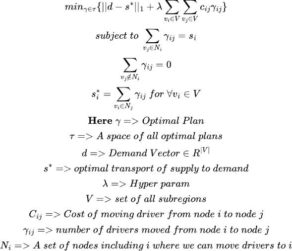
Thus, optimizing global diagnostic measures like supply-demand gap (SD) in aggregated fashion:
selecting a weight measure wᵢ and aggregating the local gaps $m_{i} = \log{s_{i}} - \log{d_{i}}$,
$A = \frac{\sum_{i=1}^{n} w_{i}\cdot m_{i}}{\sum_{i=1}^{n}w_{i}}$
where $w_{i}$ can represent business weighting, i.e. total demand in an entity $i$
We can compute a demand-centric view and a supply-centric view of the marketplace by using the corresponding weights, as proposed by Lyft:
$A_{d} = \frac{\sum_{i=1}^{n} d_{i}\cdot m_{i}}{\sum_{i=1}^{n}d_{i}}$
$A_{s} = \frac{\sum_{i=1}^{n} s_{i}\cdot m_{i}}{\sum_{i=1}^{n}s_{i}}$
Currently supported wrappers:
-
NOTE
- Works best for small $N \in [2, 500]$
- For now only dense arrays are supported (still, sparse format is accepted by SciPy and, thus, may be introduced here in the future), so beware of $O(N^2)$ memory usage!
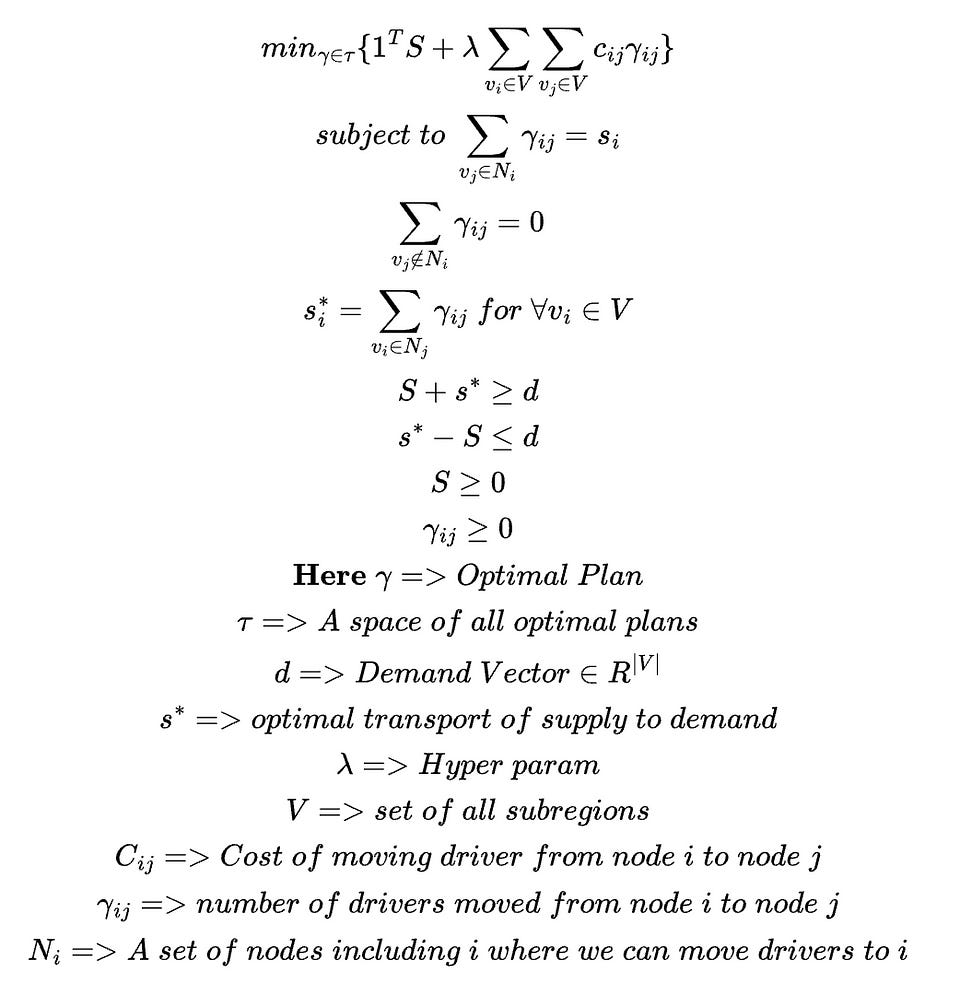
As we have L1-norm in an objective function, and many solvers (including SciPy's) do not support it, we can reformulate the problem.
Reformulating an L1-norm using additional variables and constraints involves introducing new variables to represent the absolute values of the original variables, and then adding constraints to ensure the correct relationship between the new and original variables. Here's a simple example.
Consider a linear programming problem with the following L1-norm objective function:
minimize |x1| + |x2|

Subject to:

x1 + x2 >= 1
We can reformulate the L1-norm by introducing two new sets of variables: y1 and y2, which represent the absolute values of x1 and x2, respectively. Then, we can rewrite the objective function and constraints as follows:
minimize y1 + y2

Subject to:

x1 + x2 >= 1
x1 - y1 <= 0
-x1 - y1 <= 0
x2 - y2 <= 0
-x2 - y2 <= 0
The new constraints ensure that y1 = |x1| and y2 = |x2|. The reformulated problem is now a linear programming problem without an explicit L1-norm in the objective function.
You can use this approach to reformulate L1-norms in more complex optimization problems, as long as you introduce the appropriate variables and constraints to represent the absolute values of the original variables.
So, omitting L1-norm in GEM objective will lead us to the next LP problem to solve:
Example usage
Here is an example of how to decrease supply-demand gap (SD gap), using SciPy's wrapper
n = 5
adj_matrix = create_fake_adjacency_matrix(n_nodes=n)

demand = np.array([5, 2, 3, 10, 2])
supply = np.array([3, 8, 1, 6, 5])

logger.info(f"Example of GEM optimization and supply gap reduction for fake graph with {n} nodes")
logger.info(f"\nDemand:{demand.tolist()}\nSupply:{supply.tolist()}")

sampler = np.random.RandomState(42)
c_fn = partial(fake_cost_fn, use_const=0.25, sampler=sampler)  # constant costs of magnitude 0.25
graph = nx.from_numpy_array(adj_matrix, create_using=nx.DiGraph)
graph = construct_cost_graph(graph=graph, cost_fn=c_fn, cost_field_name=DEFAULT_PARAMS["COST_FIELD_NAME"])

# nx.draw_spring(cG);  uncomment to see viz

supply_gap_init = supply_demand_gap(supply=supply, demand=demand, aggregate=True, weight_matrix=demand)
logger.info(f"Initial supply gap (aggregated): {supply_gap_init:.4f}")
# Initial supply gap (aggregated): -0.2888 - aggregated under-supply

# create optimization wrapper for scipy's linprog
opt_wrapper = ScipyWrapper(
    interaction_graph=graph,
    demand=demand,
    supply=supply,
    # other params are set to defaults, see docstring for the details
)

# see what problem we are solving (objective with dummy variables and all the constraints)
logger.info(f"Objective   (symbolic):\n{opt_wrapper.objective_symbolic}")
# min f(y,S,C,λ=2.0) = 1.0*S1 + 1.0*S2 + 1.0*S3 + 1.0*S4 + 1.0*S5
# + 0.5*y1_2 + 0.5*y2_1 + 0.5*y2_3 + 0.5*y3_2 + 0.5*y3_4 + 0.5*y4_3 + 0.5*y4_5 + 0.5*y5_4
logger.info("Constraints (symbolic):")
ineq_constraints = "\n".join(opt_wrapper.constraints_symbolic["ineq"])
logger.info(f"Inequalities:\n{ineq_constraints}")
# (-1.0)*S1 + (1.0)*y1_1 + (1.0)*y2_1 <= 5 ...
eq_constraints = "\n".join(opt_wrapper.constraints_symbolic["eq"])
logger.info(f"Equalities:\n{eq_constraints}")
# (1.0)*y1_1 + (1.0)*y1_2 = 3
logger.info(f"\nObjective   (numerical):\n{opt_wrapper.objective_numerical}")
logger.info("Constraints (numerical):")
# [1.  1.  1.  1.  1.  0.  0.5 0.5 0.  0.5 0.5 0.  0.5 0.5 0.  0.5 0.5 0. ]
ineq_constraints = "\n".join(
    [
        str(opt_wrapper.constraints_numerical["lhs_ineq"]),
        str(opt_wrapper.constraints_numerical["rhs_ineq"])
    ]
)
logger.info(f"Inequalities:\n{ineq_constraints}")
eq_constraints = "\n".join(
    [
        str(opt_wrapper.constraints_numerical["lhs_eq"]),
        str(opt_wrapper.constraints_numerical["rhs_eq"])
    ]
)
logger.info(f"Equalities:\n{eq_constraints}")

# perform optimization
# default args used here, see docstring of correspondent optimizer and pass desired set as `optimizer_kwargs` argument
opt_results = opt_wrapper.optimize()

# recalculate supply
supply_optimized = calculate_optimized_supply(
    opt_results=opt_results.x,
    symbolic_order=opt_wrapper.symbolic_order,
    idx_from=len(opt_wrapper.dummy_variables),
)

logger.info(f"Optimized supply: {supply_optimized}")
# Optimized supply: [ 5.  3.  3. 10.  2.]

supply_gap_opt = supply_demand_gap(supply=supply_optimized, demand=demand, aggregate=True, weight_matrix=demand)
logger.info(f"Optimized supply gap (aggregated): {supply_gap_opt:.4f}")
# Optimized supply gap (aggregated): 0.0369 - almost reach equilibrium
Release history Release notifications | RSS feed

Download files
Download the file for your platform. If you're not sure which to choose, learn more about installing packages.
Source Distribution
Built Distribution
Filter files by name, interpreter, ABI, and platform.
If you're not sure about the file name format, learn more about wheel file names.
Copy a direct link to the current filters
File details
Details for the file gem_opt-0.1.1.tar.gz.
File metadata
- Download URL: gem_opt-0.1.1.tar.gz
- Upload date:
- Size: 15.9 kB
- Tags: Source
- Uploaded using Trusted Publishing? No
- Uploaded via: poetry/1.4.2 CPython/3.9.13 Linux/5.19.0-38-generic
File hashes
| Algorithm | Hash digest | |
|---|---|---|
| SHA256 |
4eebceb665c5943c0bb6c0055ac21fa7f37002d2ec06af0139f9e3ed08bda830
|
|
| MD5 |
72dac6a6033811151fc382a83e05d2a4
|
|
| BLAKE2b-256 |
69e1a3c5a8623e618fd9b881919768274ecde37f24bf83888aca2d3236a5879d
|
File details
Details for the file gem_opt-0.1.1-py3-none-any.whl.
File metadata
- Download URL: gem_opt-0.1.1-py3-none-any.whl
- Upload date:
- Size: 17.3 kB
- Tags: Python 3
- Uploaded using Trusted Publishing? No
- Uploaded via: poetry/1.4.2 CPython/3.9.13 Linux/5.19.0-38-generic
File hashes
| Algorithm | Hash digest | |
|---|---|---|
| SHA256 |
1dfd09e8b4156475dc4783fe91c627d2b3e923306611597f0875a414a5d3a752
|
|
| MD5 |
f009815007b823f9af04e98a76567ff3
|
|
| BLAKE2b-256 |
d8ebe059c2171624f638e288df6efb68fe48bf63fa341815204aba64c019c7a2
|






