
Geo-trax















Geo-trax (GEO-referenced TRAjectory eXtraction) is a comprehensive pipeline that extracts high-accuracy, georeferenced vehicle trajectories from high-altitude drone imagery. Built for quasi-stationary aerial monitoring of urban traffic, it turns raw bird's-eye view (BEV) drone footage into precise, real-world vehicle trajectories. The framework combines YOLO detection, multi-object tracking, and video stabilization with a robust orthophoto-based georeferencing stage, producing GNSS-tagged, lane-resolved trajectories that are spatially and temporally consistent and ready for large-scale traffic analysis and simulation. It is optimized for urban intersections and arterial corridors, where high-fidelity, vehicle-level insights drive intelligent transportation systems and digital twin applications.

🎬 An accelerated preview of Geo-trax's capabilities. Watch the full ~4 min 4K demo on YouTube.
[!TIP] Just want to see it work? Try the interactive demo on 🤗 Hugging Face Spaces: run the vehicle detector on your own aerial image or short clip right in the browser, no install required.
Why Geo-trax
- 🛰️ Real-world output: georeferenced, lane-resolved trajectories (WGS84 + local CRS) with per-vehicle speed, acceleration, and estimated dimensions, straight from raw BEV drone video.
- 🎯 Accurate detection: YOLOv8s vehicle detector reaching 0.951 mAP@50, trained on more than 19,000 annotated aerial images.
- 🚗 Flexible tracking: four vehicle classes and six selectable multi-object trackers (BoT-SORT, ByteTrack, OC-SORT, and more).
- 🌀 Drone-motion robust: homography-based stabilization (Stabilo) plus orthophoto image registration for consistent, cross-flight coordinates; both optionally CUDA-accelerated.
- 📊 Proven at scale: powered the Songdo Traffic dataset (roughly 700,000 trajectories across 20 intersections, fleet of 10 drones; see Real-World Deployment).
- ⚙️ One command, one config:
geotrax batchruns the whole pipeline; a single YAML drives every stage, with four tuned presets included.
Pipeline

🔍 The core pipeline (solid box) produces stabilized, pixel-coordinate vehicle trajectories. Optional extensions add georeferencing via orthophoto image registration, vision dataset creation through frame (pre-)annotation for custom detector fine-tuning, and visualization, analysis, and probe vehicle validation tools, all applicable to both pixel-coordinate and georeferenced outputs.
Install
python3.11 -m venv .venv && source .venv/bin/activate  # Windows: .venv\Scripts\activate
python -m pip install geo-trax
Python 3.9 to 3.13. Also works with uv (uv pip install geo-trax) and conda. For development:
git clone --depth 1 https://github.com/rfonod/geo-trax.git
cd geo-trax && python -m pip install -e '.[dev]'
[!NOTE] The default model auto-downloads from 🤗 Hugging Face on first use (cached in
~/.cache/huggingface/hub, overridable viaHF_HOME). To use your own weights, set--modelorextraction.modelin the config to a local.ptpath orhf://<org>/<repo>/<path/to/file>.pt.
Alternative Environments & Advanced Dev Install
Create and activate a virtual environment (any of the following):
# venv (standard library)
python3.11 -m venv .venv
source .venv/bin/activate          # Windows: .venv\Scripts\activate

# uv (fastest drop-in for venv + pip)
uv venv --python 3.11
source .venv/bin/activate          # Windows: .venv\Scripts\activate

# Miniconda
conda create -n geo-trax python=3.11 -y
conda activate geo-trax
Install from PyPI (runtime use). This installs the geotrax command-line interface together with the bundled configuration tree (geotrax/cfg/):
python -m pip install geo-trax    # pip
uv pip install geo-trax           # uv (faster)
Install from local source (recommended for development or model training). Clone (or fork) the repository, then install in editable mode (-e), which reflects code changes without reinstalling:
git clone https://github.com/rfonod/geo-trax.git   # add --depth 1 for the latest snapshot only
cd geo-trax
python -m pip install -e .         # pip
# uv pip install -e .              # uv (faster; requires the uv venv above)
# poetry install                   # Poetry (auto-manages its own virtualenv; skip the venv step)
Optional dependency groups (development/testing tools, ONNX export):
python -m pip install -e '.[dev]'      # development + test tooling
python -m pip install -e '.[export]'   # ONNX export dependencies
# uv pip install -e '.[dev]'           # uv equivalents
# poetry install --extras dev          # Poetry equivalents
# poetry install --extras export
Optional CUDA for image matching. The stabilization (--stab-gpu) and georeferencing (--geo-gpu) steps can be CUDA-accelerated on top of a source-built OpenCV. Installing into such an environment needs care so the CPU OpenCV wheels do not overwrite your build; see GPU acceleration for the full setup, install-without-clobbering recipes, and a benchmark. (Object detection already uses CUDA automatically when available, via ultralytics.device.)
Quick Start
data/U_video_cut.mp4 is a 5-second sample clip included for immediate testing. See data/README.md for matching orthophotos.
# Pixel-coordinate trajectories (no orthophoto required)
geotrax batch data/U_video_cut.mp4 --no-geo

# Full pipeline: extract, georeference, and analyze (orthophotos required; see data/README.md)
geotrax batch data/U_video_cut.mp4 -orf data/orthophotos -mf data/master_frames --show-lanes

# Scale up: process a whole project tree, then merge multi-drone results into one dataset
geotrax batch path/to/PROCESSED/
geotrax aggregate path/to/PROCESSED/
Run geotrax -h or geotrax batch -h for all options. The scale-up commands above run flag-free with the recommended project structure; any other layout works with explicit path flags.
📋 Full Feature Overview
- Detection: YOLOv8s on aerial BEV imagery; detects car (incl. vans), bus, truck, and motorcycle.
- Tracking: six multi-object trackers (BoT-SORT default); see Tracking for a comparison; optional per-track frame-gap interpolation.
- Stabilization: homography-based trajectory correction via Stabilo 🌀, tuned with Stabilo-Optimize 🎯; optional CUDA acceleration (
--stab-gpu). - Georeferencing: frame-to-orthophoto registration; outputs lat/lon, local CRS, speed, acceleration, and lane assignment per vehicle; optional CUDA acceleration (
--geo-gpu). - Visualization: track overlays on original, stabilized, or static-reference video, in five rendering modes (incl. oriented bounding boxes).
- Analysis: trajectory maps, kinematic distributions, and class/dimension charts, per-video or aggregated across drones and sessions.
- Scaling & tooling: batch-processes directory trees and aggregates multi-drone data; includes standalone utilities for end-to-end data preparation, training, evaluation, and validation.
🚀 Planned Enhancements
- Comprehensive documentation in a dedicated
docs/folder. Atools/README.mdindex already covers the auxiliary scripts. - Modularized, OOP-based pipeline with custom reference frame support and georeferencing leveraging Stabilo's image-matching backend.
- Per-class confidence thresholds.
- SAHI-based small-object detection.
- Batch inference and multi-thread processing.
- Real-world map visualization (e.g., MovingPandas, contextily) and interactive web app.
🔗 Related Projects
Geo-trax integrates with and complements several specialized tools:
-
Stabilo 🌀: Python library for video and trajectory stabilization using robust homography transformations. Supports various feature detectors, RANSAC algorithms, and user-defined masks. Used as Geo-trax's core stabilization engine.
-
Stabilo-Optimize 🎯: benchmarking and hyperparameter optimization framework for Stabilo. Evaluates stabilization performance through ground truth-free assessment using random perturbations. Used to fine-tune Geo-trax stabilization parameters.
-
HBB2OBB 📦: converts horizontal bounding boxes to oriented bounding boxes using SAM segmentation models. Can enhance Geo-trax outputs when object orientation is needed for downstream analysis.
Configuration
The entire pipeline is driven by a single, self-contained YAML config: one file for detection, tracking, stabilization, georeferencing, visualization, and plotting. Four presets ship with the package:
| Preset | Focus |
|---|---|
default |
Balanced baseline |
confident |
Precision (fewer false positives) |
lenient |
Recall (catches more vehicles) |
stable |
Stabilization quality |
geotrax batch video.mp4 -c confident   # use a bundled preset by name
geotrax batch video.mp4 -c ./my.yaml   # use a custom config file
⚙️ Inspect, copy, and customize configs
Manage the bundled configs with the geotrax config command:
geotrax config show              # list bundled presets and their location
geotrax config show default      # print a preset's full contents
geotrax config copy              # copy presets into the current directory as <name>_copy.yaml
geotrax config copy -o ~/myproj  # copy into a specific directory
Copy a preset, edit it, then pass it with -c:
geotrax config copy
# edit default_copy.yaml ...
geotrax extract video.mp4 -c default_copy.yaml
To switch the tracking algorithm, set tracker.active in the config (see Tracking).
GPU acceleration
Object detection already runs on CUDA automatically whenever a compatible GPU and PyTorch build are present (via the ultralytics.device config key, auto by default). The stabilization (--stab-gpu) and georeferencing (--geo-gpu) image-matching steps can optionally be CUDA-accelerated too, through Stabilo 1.3.0+. This needs a CUDA-enabled OpenCV build and is Linux/Windows only. Stabilo accelerates the ORB detector only, so --geo-gpu additionally requires georef.matching.detector_name: orb; there is no CPU fallback, so requesting GPU without a working CUDA device raises an error.
⚡ Full CUDA setup & benchmarking guide
Throughout this guide, dotted names like ultralytics.device or georef.matching.detector_name are keys in the pipeline config, not CLI flags. To change them, copy the bundled config once and pass your copy with -c:
geotrax config copy                 # writes default_copy.yaml in the current directory
# edit default_copy.yaml, then pass it to any command:
geotrax batch <video> ... -c default_copy.yaml
1. Build OpenCV with CUDA
The PyPI OpenCV wheels are CPU-only, so you must build opencv-contrib-python from source with CUDA. Follow Stabilo's docs/cuda.md, then confirm it works:
python -c "import cv2; print(cv2.__version__, cv2.cuda.getCudaEnabledDeviceCount())" # expect: <version> 1
geo-trax needs one OpenCV module beyond the minimal stabilo build: add
videoto theBUILD_LIST. The minimal list in stabilo's guide omits it, but thesparseOptFlowglobal-motion-compensation (GMC) method usescv2.calcOpticalFlowPyrLKfrom that module. It is the default for the BoT-SORT (active default) and TrackTrack trackers, and an option for DeepOCSORT (tracker.<name>.gmc_method). GMC runs during track association on the original, pre-stabilization frames, so Stabilo does not make it redundant. Withoutvideoyou get acv2 has no attribute 'calcOpticalFlowPyrLK'warning and GMC silently falls back to identity. If you would rather not rebuild, setgmc_method: nonefor your active tracker (step 3), but that disables camera-motion compensation in tracking; for near-nadir BEV / quasi-stationary drone footage that is often acceptable, but check your tracking quality before relying on it.
2. Install geo-trax without clobbering your CUDA OpenCV
ultralytics[extra] transitively requires opencv-python and opencv-python-headless, both CPU wheels. A plain install drops them on top of your compiled cv2/ and disables CUDA. A transitive dependency cannot be excluded in pyproject.toml, so use one of these:
A. Install, then restore your wheel (recommended). Let pip install everything, then overwrite the CPU OpenCV by reinstalling the CUDA opencv_contrib_python-*.whl you built in step 1:
pip install -e .          # installs torch/cuda/ultralytics/..., plus (temporarily) CPU opencv
# reinstall the wheel produced by your CUDA OpenCV build in step 1 (path is wherever you built it):
pip install --force-reinstall --no-deps /path/to/opencv_contrib_python-*.whl
python -c "import cv2; print(cv2.cuda.getCudaEnabledDeviceCount())"   # expect: 1
If the CUDA check above reports
0devices (or acv2/CUDA error such asmodule 'cv2' has no attribute 'cuda') immediately after the reinstall, re-activate the CUDA venv (source .venv-cuda/bin/activate, matching stabilo'sdocs/cuda.md) and run it again; if it persists, confirmcv2.__file__points into that venv'ssite-packages(see the troubleshooting in stabilo'sdocs/cuda.md). It should then report1.⚠️ Afterwards
opencv-python/opencv-python-headlessstay registered but their recorded files now belong to your build. Neverpip uninstall opencv-python/opencv-python-headless, or you will delete the sharedcv2/.
B. Stub the CPU wheels first (no download, cleaner metadata). Install two metadata-only packages so pip treats the requirements as already satisfied and never fetches a CPU wheel:
CVVER=$(python -c "import cv2; print(cv2.__version__)")
for pkg in opencv-python opencv-python-headless; do
  d=$(mktemp -d)
  cat > "$d/pyproject.toml" <<EOF
[build-system]
requires = ["setuptools"]
build-backend = "setuptools.build_meta"
[project]
name = "$pkg"
version = "$CVVER"
[tool.setuptools]
py-modules = []
EOF
  pip install --no-deps "$d" && rm -rf "$d"
done
pip install -e .          # opencv is satisfied by the stubs; your CUDA build is untouched
3. Enable GPU per stage
| Stage | How | Notes |
|---|---|---|
| Detection | automatic | ultralytics.device (auto = CUDA when available) |
| Stabilization | --stab-gpu |
works out of the box (default detector is ORB) |
| Georeferencing | --geo-gpu + detector_name: orb |
set via a copied config (below) |
Only ORB is CUDA-accelerated, and the georeferencing detector is not a CLI flag, so enable georef GPU through a copied config:
geotrax config copy                       # writes default_copy.yaml
# edit default_copy.yaml:
#   georef.matching.detector_name: orb    # required for --geo-gpu
#   tracker.botsort.gmc_method: none      # ONLY if you did not add 'video' to BUILD_LIST (step 1); disables tracker GMC, verify tracking quality
These are the GPU-accelerated analogues of the two reproduce commands in data/README.md. Their outputs are equivalent, not identical to the committed data/results-pixel/ and data/results-full/: the CUDA path georeferences with ORB (RootSIFT is not GPU-accelerated), GPU feature extraction is not bit-identical to CPU, and with gmc_method: none the tracker runs without motion compensation.
# Pixel-coordinate results: GPU stabilization, no georeferencing
geotrax batch data/U_video_cut.mp4 --no-geo --show-class-names --show-conf --stab-gpu -c default_copy.yaml

# Full pipeline: GPU stabilization + georeferencing (needs the orthophoto/segmentation/master-frame data; see data/README.md)
geotrax batch data/U_video_cut.mp4 -orf data/orthophotos -osf data/segmentations -mf data/master_frames \
  --show-lanes --plot-segmentations -vm 0 3 --stab-gpu --geo-gpu -c default_copy.yaml
4. Benchmark: detection-only CUDA vs fully CUDA
To isolate the GPU effect, disable the CPU-bound visualization and plotting (--no-save --no-show --no-plot-save --no-plot-show) and wipe a scratch output folder before each run (a clean, non-skipped run that leaves your real results untouched). Do not pass --recompute: the master→orthophoto homography is a one-time, expensive registration normally cached in the master-frames folder, so leaving it cached keeps the benchmark on the per-video work (detection, stabilization, reference→master registration).
Three configurations are compared:
- geo-trax default (CPU): the shipped defaults with RootSIFT georeferencing; what a CPU-only user actually runs.
- ORB (CPU): the GPU-tuned config on CPU; a controlled, same-config baseline for the GPU run.
- fully CUDA: the same ORB config with
--stab-gpu --geo-gpu.
The default run needs no config file: with no -c, geo-trax uses its shipped defaults (RootSIFT georeferencing, CPU for both stabilization and georeferencing). The ORB runs use your default_copy.yaml (georef.matching.detector_name: orb, tracker.botsort.gmc_method: none).
With hyperfine:
OUT=/tmp/geotrax_bench
COMMON="geotrax batch data/U_video_cut.mp4 -orf data/orthophotos -osf data/segmentations -mf data/master_frames --no-save --no-show --no-plot-save --no-plot-show -of $OUT"
hyperfine --warmup 1 --runs 5 --prepare "rm -rf $OUT" \
  -n "geo-trax default (CPU, RootSIFT)" "$COMMON" \
  -n "ORB (CPU)"                        "$COMMON -c default_copy.yaml" \
  -n "fully CUDA (ORB)"                 "$COMMON -c default_copy.yaml --stab-gpu --geo-gpu"
Or without extra tools:
bench () { local label="$1"; shift; rm -rf /tmp/geotrax_bench
  local t0=$(date +%s.%N)
  geotrax batch data/U_video_cut.mp4 -orf data/orthophotos -osf data/segmentations -mf data/master_frames \
    --no-save --no-show --no-plot-save --no-plot-show -y -o -of /tmp/geotrax_bench "$@" >/tmp/bench.log 2>&1 \
    && awk -v a="$t0" -v b="$(date +%s.%N)" -v l="$label" 'BEGIN{printf "%-28s %.1f s\n", l, b-a}' \
    || echo "$label FAILED (see /tmp/bench.log)"; }
bench "geo-trax default (CPU)"
bench "ORB (CPU)"        -c default_copy.yaml
bench "fully CUDA (ORB)" -c default_copy.yaml --stab-gpu --geo-gpu
Example on an NVIDIA RTX 4090 (5-second sample clip, 150 frames; hyperfine mean ± σ over 5 runs):
Benchmark system
- OS: Ubuntu 24.04.4 LTS (Linux 6.8, x86_64)
- CPU: 13th Gen Intel Core i9-13900KF (24 cores / 32 threads)
- RAM: 62 GiB
- GPU: NVIDIA GeForce RTX 4090 (24 GB, driver 580.159.03)
- Software: Python 3.11.5, torch 2.12.1 (CUDA 13.0), OpenCV 4.13.0, stabilo 1.3.0
| Pipeline | Wall time | vs default |
|---|---|---|
| CPU stabilization and georeferencing (geo-trax defaults) | 273.7 ± 0.9 s | 1× |
| CPU stabilization and georeferencing (GPU-matched config) | 348.4 ± 0.4 s | 0.8× |
| Fully CUDA (GPU-matched config) | 16.4 ± 2.0 s | 16.7× |
Fully CUDA is 16.7× faster than the geo-trax default and 21.3× faster than the same ORB config on CPU (row 2). Row 1 is the shipped defaults (RootSIFT georeferencing); rows 2–3 use the GPU-matched config, which switches georeferencing to ORB so the CPU and GPU runs do identical work (only ORB is CUDA-accelerated). Row 2 is slower than row 1 because ORB at a 250k feature ceiling with brute-force matching is costlier on CPU than RootSIFT. Treat these as a relative comparison, not absolute throughput: geo-trax's defaults favor maximum accuracy and reliability, with detection at 1920×1920, stabilization at only a 0.5 downscale (roughly 2K per frame on this 4K clip) with a high
max_featuresceiling, and RootSIFT georeferencing with a very highmax_featuresand conservative MAGSAC++ matcher/projection settings, all against an 8000×8000 orthophoto. Lighter settings would cut absolute times across the board; the point is the CPU→GPU ratio.
Detection Model
The default detector is YOLOv8s (HBB, 1920 × 1920 px, ~11 M parameters), trained on more than 19,000 annotated aerial images (~679k labeled vehicle instances) and fine-tuned on a curated, high-quality subset. It is hosted on 🤗 Hugging Face and downloads automatically on first use. Results on the Songdo Vision test split (1,084 images; full results in Table 3):
| ID | Label | Precision | Recall | mAP@50 | mAP@50-95 |
|---|---|---|---|---|---|
| 0 | Car (incl. vans) | 0.979 | 0.981 | 0.992 | 0.835 |
| 1 | Bus | 0.952 | 0.977 | 0.988 | 0.826 |
| 2 | Truck | 0.887 | 0.916 | 0.935 | 0.722 |
| 3 | Motorcycle | 0.827 | 0.866 | 0.888 | 0.463 |
| All | 0.911 | 0.935 | 0.951 | 0.711 |
Pedestrian and bicycle classes exist in the weights but are underrepresented, unevaluated, and filtered by default. See the model card for full details.
To use a different model, point --model (CLI) or extraction.model (config) to a local .pt path or hf://<org>/<repo>/<file>.pt; any Ultralytics-compatible model works.
Custom Model Training
Training and export scripts for custom YOLO detectors live in train/, with a SLURM wrapper for HPC clusters. See train/README.md.
Tracking
Six multi-object trackers ship with Ultralytics >=8.4.63. Selection is config-driven: set tracker.active, no code changes needed. Default: BoT-SORT.
| Tracker | tracker.active |
ReID | GMC¹ | Pros | Cons |
|---|---|---|---|---|---|
| BoT-SORT (default) | botsort |
opt | ✅ | Strong accuracy; motion + optional appearance | Slower; ReID adds compute |
| ByteTrack | bytetrack |
❌ | ❌ | Fastest; two-stage association | More ID switches under occlusion |
| OC-SORT | ocsort |
❌ | ❌ | Robust to non-linear motion; lightweight | Weaker on long occlusions |
| Deep OC-SORT | deepocsort |
opt | opt | OC-SORT + appearance; dense scenes | Heaviest variant with ReID |
| FastTracker | fasttrack |
❌ | ❌ | Occlusion-aware ByteTrack variant | Newer; several knobs to tune |
| TrackTrack | tracktrack |
opt | ✅ | Multi-cue cost; best ID retention | Most parameters; highest compute |
¹ GMC (in-tracker camera-motion compensation) runs during tracking and is independent of Stabilo's post-hoc trajectory stabilization stage.
💡 Run
geotrax config show defaultto print the fulltracker:block, with every parameter for all six trackers documented inline. Rungeotrax config copyto get an editable local copy. For a head-to-head comparison on your own data, seetools/compare_tracking.py.
Usage
The geotrax CLI provides one subcommand per stage: batch (primary entry point), extract, georeference, visualize, plot, aggregate, and config. Run geotrax -h or geotrax <subcommand> -h for the full reference (python -m geotrax works identically).
# Recursively process a directory (or a single video) without georeferencing
geotrax batch path/to/videos/ --no-geo

# Run an individual stage on its own
geotrax extract video.mp4                  # detect, track, and stabilize
geotrax visualize video.mp4 --save         # render an annotated video from existing results
geotrax plot video.mp4                     # trajectory and distribution plots
[!TIP] See data/README.md for sample data and testing examples.
💡 More Examples & Advanced Usage
# Use a custom config (bundled preset by name, or a path to your own file)
geotrax batch video.mp4 -c confident
geotrax batch video.mp4 -c path/to/custom_config.yaml

# Fill per-track detection gaps with linear interpolation (adds is_interpolated column to .txt output)
geotrax batch video.mp4 --no-geo --interpolate

# Regenerate visualization without re-running extraction
geotrax batch video.mp4 --viz-only --save

# Show lane IDs, hide the speed overlay (requires georeferencing)
geotrax batch video.mp4 --viz-only --save --show-lanes --hide-speed

# Georeference an already-extracted video against orthophotos
geotrax georeference video.mp4 -orf path/to/orthophotos -mf path/to/master_frames

# Aggregated trajectory plots, excluding buses and trucks
geotrax batch path/to/PROCESSED/ --plot-only --plot-aggregate --plot-class-filter 1 2

# Merge multi-drone results for the same locations into a unified dataset
geotrax aggregate path/to/PROCESSED/

# Rotated box modes (3/4): boxes oriented to vehicle heading, on original (3) or stabilized (4) frame
geotrax visualize video.mp4 --save --viz-mode 3 4
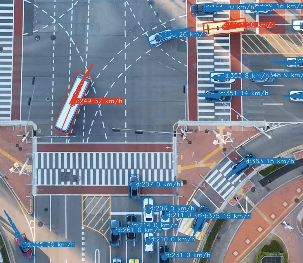
Mode 3 rotated bounding boxes, zoomed detail from the same scene as the animation above.
⚠️ Rotated box modes (3 and 4): known limitations
Modes 3 and 4 replace the standard axis-aligned YOLO detections with rotated bounding boxes: each box is sized to the vehicle's estimated physical length and width and rotated to align with its travel direction (heading). The heading is derived from the camera-motion-free stabilized trajectory; mode 3 projects the result back onto the original frame, while mode 4 draws directly on the stabilized frame. They are the most informative rendering modes but also the most sensitive to data quality:
- Size estimation may fail. Estimates are computed over frames where the vehicle moves in a nearly straight path with sufficient displacement. Short tracks, near-stationary vehicles, or detections close to the frame edges can yield no usable estimate. In those cases the box dimensions fall back to a per-vehicle Q25 aggregate of the raw YOLO bounding box extents (rotated to the heading), which tends to be inflated during turns since axis-aligned detections expand as the vehicle turns. Fallback boxes are rendered with a dashed outline so they are easy to identify.
- Heading may be unreliable. For very slow or stationary vehicles the motion direction cannot be determined; the box is then aligned with the longer axis of the raw bounding box instead.
- Back-projection distortion (mode 3 only). Oriented boxes are computed in stabilized space and projected back onto the original frame via the inverse stabilization homography. Under strong camera motion this can produce visibly skewed boxes.
- Edge clipping is approximate. When a vehicle is entering or exiting the frame, the detection only covers its visible part, so the oriented box is clipped to that footprint instead of being drawn at full size (the clip is triggered once the detection reaches within
edge_clip_marginpixels of the border, since the YOLO box may stop a few pixels short of the true edge). That footprint, however, is only known as an axis-aligned (HBB) detection box, whereas the rendered box is rotated to the heading — so the clip boundary only approximates where the rotated vehicle actually leaves the frame. The clip rectangle is temporally smoothed (edge_clip_smoothing) so the box shrinks steadily as the vehicle exits rather than jumping with per-frame detection noise. - Both modes require that the extraction stage was run with stabilization enabled (
stabilize: truein the config).
[!NOTE] Why use master frames? When georeferencing, geo-trax can route each video's homography through a shared master frame per location ID. A master frame is a high-quality, near-nadir BEV frame chosen once per location (see
tools/find_master_frames.py), used instead of registering every video's reference frame directly to the orthophoto. The mapping is split into two homographies:reference → master(recomputed per video) andmaster → orthophoto(computed once per location ID and cached, validated by a hash of the master image). This gives two benefits:
- Speed: the expensive cross-domain
master → orthophotoregistration runs once and is reused across every drone and flight at that location, instead of once per video.- Consistency & robustness: every video is matched against the same master frame. This same-modality BEV-to-BEV registration is far more reliable than a direct BEV-to-orthophoto match, so trajectories from different drones, altitudes, and viewpoints resolve into one coherent coordinate system.
Master frames are enabled by default. Disable them with
--no-master, or force re-computation of the cachedmaster → orthophotohomography with--recompute.
📁 Output file formats
Suppose the input video is video_file.mp4. By default, outputs are written to a results/ sub-folder next to the input; the folder and all filename postfixes are configurable via the output: section of the pipeline config (or --output-folder / -of for the folder).
-
video_file.txt (
<stem><tracks_postfix>.txt): Contains the extracted vehicle trajectories in the following format:frame_id, vehicle_id, x_c(unstab), y_c(unstab), w(unstab), h(unstab), x_c(stab), y_c(stab), w(stab), h(stab), class_id, confidence, vehicle_length, vehicle_width
where:
frame_id: Frame number (0, 1, ...).vehicle_id: Unique vehicle identifier (1, 2, ...).x_c(unstab),y_c(unstab): Unstabilized vehicle centroid coordinates.w(unstab),h(unstab): Unstabilized vehicle bounding box width and height.x_c(stab),y_c(stab): Stabilized vehicle centroid coordinates.w(stab),h(stab): Stabilized vehicle bounding box width and height.class_id: Vehicle class identifier (0: car (incl. vans), 1: bus, 2: truck, 3: motorcycle)confidence: Detection confidence score (0-1).vehicle_length,vehicle_width: Estimated vehicle dimensions in pixels.is_interpolated(optional, 15th column): Present only whenextraction.interpolate: true(CLI:--interpolate).0= real detection,1= linearly interpolated to fill a frame gap. Gaps larger than the active tracker'strack_bufferare left unfilled (the tracker would not persist a lost track's ID across a longer occlusion).
-
video_file_vid_transf.txt (
<stem><stab_transform_postfix>.txt): Contains the transformation matrix for each frame in the format:frame_id, h11, h12, h13, h21, h22, h23, h31, h32, h33
where:
frame_id: Frame number of the stabilized frame (starts fromcut_frame_left + 1since the reference frame itself has no transform).hij: Elements of the 3x3 homography matrix that maps each frame (frame_id) to the reference frame.
-
video_file.yaml: Video metadata and the configuration settings used for processing
video_file.mp4. (This file is saved in the same directory as the input video, not in the output folder.) -
video_file_mode_X.mp4 (
<stem><visualization_postfix>_mode_<X>.mp4): Annotated video in five rendering modes (X = 0 / 1 / 2 / 3 / 4):- Mode 0: overlaid on the original (unstabilized) video
- Mode 1: overlaid on the stabilized video
- Mode 2: plotted on the static reference frame
- Mode 3: rotated bounding boxes on the original video, where each box is sized to the vehicle's estimated physical dimensions and rotated to its per-frame heading (derived from the camera-motion-free stabilized trajectory and projected back onto the original frame). Requires stabilization to have been run.
- Mode 4: the same rotated bounding boxes as Mode 3, but drawn directly on the stabilized video (no back-projection). Requires stabilization to have been run.
Each version can display vehicle bounding boxes, IDs, class labels, confidence scores, and short trajectory trails that fade and vary in thickness to indicate the recency of the movement. If an input
video_file.csvfile is available in the same directory as the input video, i.e., the converted flight logs, vehicle speed and lane information can also be displayed. -
video_file.csv (
<stem><georeferenced_postfix>.csv): Contains the georeferenced vehicle trajectories in a tabular format. This file includes both geographic and local coordinates, estimated real-world dimensions, kinematic data, road section, and lane information. The columns are:Vehicle_ID, [Timestamp,] Frame_Number, Ortho_X, Ortho_Y, Local_X, Local_Y, Latitude, Longitude, Vehicle_Length, Vehicle_Width, Vehicle_Class, Vehicle_Speed, Vehicle_Acceleration, Road_Section, Lane_Number, Visibility[, Is_Interpolated]
where:
Vehicle_ID: Unique vehicle identifier.Timestamp: Timestamp of the frame (YYYY-MM-DD HH:MM:SS.ms). Present only when a flight-log CSV with timestamps is available alongside the video.Frame_Number: Video frame index corresponding to this detection.Ortho_X,Ortho_Y: X and Y coordinates of the vehicle centroid in the orthophoto's pixel coordinate system.Local_X,Local_Y: X and Y coordinates of the vehicle centroid in a local projected coordinate system (e.g., EPSG:5186 for KGD2002 / Central Belt 2010 used in the Songdo experiment).Latitude,Longitude: Geographic coordinates of the vehicle centroid (WGS84).Vehicle_Length,Vehicle_Width: Estimated vehicle dimensions in meters.Vehicle_Class: Vehicle class identifier (0: car (incl. vans), 1: bus, 2: truck, 3: motorcycle).Vehicle_Speed: Estimated vehicle speed in km/h.Vehicle_Acceleration: Estimated vehicle acceleration in m/s$^2$.Road_Section: Identifier for the road segment the vehicle is on.Lane_Number: Identifier for the lane the vehicle is in.Visibility: Boolean indicating if the vehicle's bounding box is fully visible within the frame.Is_Interpolated(optional): Present only when extraction was run with--interpolate(extraction.interpolate: true).0= real detection,1= row synthesized by linear interpolation at the extraction stage to fill a frame gap; propagated from the.txttracks file.
-
video_file_geo_transf.txt (
<stem><geo_transform_postfix>.txt): Contains the 3x3 georeferencing transformation matrix (homography) that maps points from the video's reference frame to the orthomap. The format is a comma-separated list of the 9 matrix elements:h11, h12, h13, h21, h22, h23, h31, h32, h33
Note: All output files (except video_file.yaml) are saved in the configured output folder (default: results/ sub-folder next to the input video). Trajectory and distribution plots are always written to a plots/ sub-folder inside the output folder.
Real-World Deployment: The Songdo Experiment
Geo-trax was validated in a large-scale urban traffic monitoring campaign in Songdo, South Korea, where it processed footage from a fleet of 10 drones to produce the Songdo Traffic dataset. The detection model was trained on the companion Songdo Vision dataset. Both are described in the publication.
| Songdo campaign | |
|---|---|
| 📍 Location | Songdo International Business District, South Korea |
| 📅 Duration | 4 days (October 4 to 7, 2022) |
| 🚁 Fleet | 10 drones (DJI Mavic 3), 140 to 150 m altitude, 4K at 29.97 fps |
| 🔭 Coverage | 20 busy intersections |
| 🚗 Result | ~700,000 georeferenced vehicle trajectories |
🎥 Demo of Geo-trax applied to the Songdo experiment: https://youtu.be/gOGivL9FFLk
The blocks below document the project layout and data-wrangling workflow used in that campaign; they double as the recommended setup for your own multi-drone projects.
📂 Recommended project folder structure
The layout below mirrors the Songdo experiment and matches the pipeline's auto-detection defaults, letting geotrax batch run with no path flags. Two conventions do the heavy lifting:
- A
PROCESSED/folder anchors auto-detection. When georeferencing or plotting needs orthophotos, master frames, or segmentations and no explicit path is given, Geo-trax walks up from the video until it findsPROCESSED, then looks for a siblingORTHOPHOTOS/folder. - A location ID ties each video to its assets. The location ID is the leading letters in the clip filename (
A1.mp4→A), soA1.mp4automatically resolves toORTHOPHOTOS/A.png,ORTHOPHOTOS/master_frames/A.png, andORTHOPHOTOS/segmentations/A.csv.
Directory tree
<project>/                                 # project root (name arbitrary)
├── RAW/                                   # untouched drone footage + flight logs (never modified)
│   └── 2022-10-07/D1/PM1/                 # arbitrary nesting, e.g. date / drone / session
│       ├── DJI_0001.MP4  DJI_0001.SRT
│       └── DJI_0002.MP4  DJI_0002.SRT     # drone splits a recording into segments (file-size limit)
├── PROCESSED/                             # pipeline input (auto-detect anchor)
│   └── 2022-10-07/D1/PM1/
│       ├── 0_merged.mp4  0_merged.srt     # merged flight video + log (temporary, deletable)
│       ├── 0_merged.txt                   # cut list: start/end frames, one cut per line (temporary)
│       ├── A1.mp4  A1.csv                 # cut clip + flight log; 'A' = location ID, '1' = sequence
│       ├── A2.mp4  A2.csv                 # next clip at the same location
│       ├── A1.yaml                        # run metadata, saved next to the clip (not in results/)
│       └── results/                       # pipeline outputs, written next to each clip
│           ├── A1.txt                     # pixel-coordinate tracks
│           ├── A1_vid_transf.txt          # stabilization homographies
│           ├── A1_geo_transf.txt          # georeferencing homography
│           ├── A1.csv                     # georeferenced trajectories + kinematics
│           ├── A1_mode_0.mp4              # video with overlaid boxes & trajectories (modes 0/1/2/3/4)
│           └── plots/                     # various trajectory & distribution plots
├── ORTHOPHOTOS/                           # auto-detected sibling of PROCESSED / DATASET
│   ├── A.png                              # orthophoto cut-out, per location
│   ├── A.txt  (or A.tif)                  # georeferencing parameters (or a georeferenced GeoTIFF)
│   ├── ortho_parameters.txt               # (alternative) shared params + per-location A_center.txt
│   ├── master_frames/                     # optional; consistent reference frame per location
│   │   ├── A.png                          #   reference frame image
│   │   └── A.txt                          #   cached master->ortho homography
│   └── segmentations/                     # optional; per-location lane/road geometry
│       ├── A.csv                          #   lane & road-section polygons
│       └── A.png                          #   overlay image (used for plotting only)
└── DATASET/                               # `geotrax aggregate` output (sibling of PROCESSED)
    └── 2022-10-07_A/                      # one intersection-day
        ├── 2022-10-07_A_AM1.csv           # one CSV per flight session (AM1-AM5, PM1-PM5),
        └── 2022-10-07_A_PM1.csv           #   trajectories merged across drones for that session
RAW/ is kept immutable; everything downstream lives under PROCESSED/. The master_frames/ and segmentations/ sub-folders are optional; provide them only when you need cross-flight georeferencing consistency or lane-level analysis. DATASET/ is created by geotrax aggregate and is also a valid auto-detection anchor for ORTHOPHOTOS/.
🏷️ Clip naming conventions
Only the leading location letters of a clip filename are required by the code (parsed by determine_location_id). The contextual metadata (date, drone, session) normally lives in the folder path, so each clip can be named compactly as location ID + sequence number:
2022-10-07/D10/PM5/U1.mp4
│          │   │   └── clip: location ID 'U' + sequence number '1'
│          │   └────── flight session: AM1-AM5 (morning) / PM1-PM5 (afternoon)
│          └────────── drone ID (D1, D2, ...)
└───────────────────── capture date (ISO 8601, YYYY-MM-DD)
These compact names are assigned automatically by the cutting step, not typed by hand: given a location map (a JSON file pairing each label with its [lat, lon] center), tools/cut_merged_videos_and_logs.py labels every clip with the location nearest to its GPS centroid and appends a per-location sequence number (U1, U2, ...).
Because only the leading letters matter, the same context can instead be packed into a single self-contained filename when clips are detached from this tree. This is how the sample videos published on Zenodo are named, e.g. U_D10_2022-10-07_PM5_60s.mp4 (location U, drone D10, date 2022-10-07, session PM5). Here the per-location sequence number is replaced by a time marker showing where the clip falls within the session: 60s denotes the first 60 seconds of that session at the location. Either way, the code still extracts location U.
| Clip filename | Location ID | Resolves to |
|---|---|---|
U1.mp4 |
U |
ORTHOPHOTOS/U.png, master_frames/U.png, segmentations/U.csv |
U2.mp4 |
U |
ORTHOPHOTOS/U.png, … |
U_D10_2022-10-07_PM5_60s.mp4 |
U |
ORTHOPHOTOS/U.png, … |
geotrax aggregate groups results by location (and date/session), merging clips from different drones that cover the same place into a unified dataset.
🛠️ From raw footage to trajectories
The tools/ directory provides the wrangling scripts that take you from raw footage to pipeline-ready clips (see tools/README.md for the full index):
- Merge the recorded video segments and their logs into one video + log per flight session →
tools/merge_videos_and_logs.py - Cut each merged flight into per-location clips: list the start/end frames of each stable hover in
0_merged.txt, then split (converting the DJI SRT log to a per-clip CSV) →tools/cut_merged_videos_and_logs.py - QA / repair the cut logs →
tools/find_cut_video_issues.py,tools/fix_timestamp_anomalies.py,tools/interpolate_missing_timestamps.py - Build the georeferencing assets: orthophoto cut-outs per location →
tools/subset_orthophoto.py; master frames →tools/find_master_frames.py; lane segmentations are drawn manually, with overlays rendered viatools/viz_segmentations.py - Run the pipeline:
geotrax batch PROCESSED/ ...; orthophotos, master frames, and segmentations are auto-detected from the siblingORTHOPHOTOS/folder. - (Optional) Aggregate results across drones and flights for the same location →
geotrax aggregate PROCESSED/, which writes a unified dataset to a siblingDATASET/folder.
Lessons from the Songdo experiment
- Treat
RAW/as read-only archival storage and derive everything underPROCESSED/; the wrangling steps are reproducible from the raw footage. - The master frame is an intermediary coordinate system per location: aligning every flight to one shared reference frame keeps trajectories from different drones, altitudes, and viewpoints in a single consistent coordinate system.
- Coordinates were projected to a local CRS (EPSG:5186, KGD2002 / Central Belt 2010) alongside WGS84 lat/lon; set your own CRS in the
georef:config section. - Imagery was captured at ~140–150 m altitude in 4K, giving a ground sampling distance of ≈ 0.027 m/px (the default
extraction.gsd). Re-tune the GSD for different altitudes or cameras.
Citation
If you use Geo-trax in your research or software, please cite:
-
Journal article (preferred for any use of the framework):
@article{fonod2025advanced,
  title = {Advanced computer vision for extracting georeferenced vehicle trajectories from drone imagery},
  author = {Fonod, Robert and Cho, Haechan and Yeo, Hwasoo and Geroliminis, Nikolas},
  journal = {Transportation Research Part C: Emerging Technologies},
  volume = {178},
  pages = {105205},
  year = {2025},
  publisher = {Elsevier},
  doi = {10.1016/j.trc.2025.105205},
  url = {https://doi.org/10.1016/j.trc.2025.105205}
}
-
Software archive (when referencing or building on the code itself):
@software{fonod2026geo-trax,
  author = {Fonod, Robert},
  title = {Geo-trax: A Comprehensive Framework for Georeferenced Vehicle Trajectory Extraction from Drone Imagery},
  year = {2026},
  month = jul,
  version = {1.2.0},
  doi = {10.5281/zenodo.12119542},
  url = {https://github.com/rfonod/geo-trax},
  license = {MIT}
}
Contributions
Early code received key contributions from Haechan Cho (georeferencing) and Sohyeong Kim (video/flight-log merging). Community contributions are welcome: open a GitHub Issue or submit a pull request.
License
This project is distributed under the MIT License. See the LICENSE for more details.
1 maintainer

Download files
Download the file for your platform. If you're not sure which to choose, learn more about installing packages.
Source Distribution
Built Distribution
Filter files by name, interpreter, ABI, and platform.
If you're not sure about the file name format, learn more about wheel file names.
Copy a direct link to the current filters
File details
Details for the file geo_trax-1.2.0.tar.gz.
File metadata
- Download URL: geo_trax-1.2.0.tar.gz
- Upload date:
- Size: 187.4 kB
- Tags: Source
- Uploaded using Trusted Publishing? Yes
- Uploaded via: twine/6.1.0 CPython/3.13.12
File hashes
| Algorithm | Hash digest | |
|---|---|---|
| SHA256 |
15aff963afd244743fd70aaeb1ff67914393ab7422fe86cb0d3cb4dfa605f7d2
|
|
| MD5 |
ef9a18173f2f830300328066c03723c9
|
|
| BLAKE2b-256 |
b5feaac98e2fe969b596e8104676deab3c0f1b49a2909cefb5f95d1d0c968d68
|
Provenance
The following attestation bundles were made for geo_trax-1.2.0.tar.gz:
Publisher:
publish.yml on rfonod/geo-trax
-
Statement:
-
Statement type:
https://in-toto.io/Statement/v1 -
Predicate type:
https://docs.pypi.org/attestations/publish/v1 -
Subject name:
geo_trax-1.2.0.tar.gz -
Subject digest:
15aff963afd244743fd70aaeb1ff67914393ab7422fe86cb0d3cb4dfa605f7d2 - Sigstore transparency entry: 2066386963
- Sigstore integration time:
-
Permalink:
rfonod/geo-trax@433764f4bf15e59a526ef4ebc4c07105e6acbd87 -
Branch / Tag:
refs/tags/v1.2.0 - Owner: https://github.com/rfonod
-
Access:
public
-
Token Issuer:
https://token.actions.githubusercontent.com -
Runner Environment:
github-hosted -
Publication workflow:
publish.yml@433764f4bf15e59a526ef4ebc4c07105e6acbd87 -
Trigger Event:
release
-
Statement type:
File details
Details for the file geo_trax-1.2.0-py3-none-any.whl.
File metadata
- Download URL: geo_trax-1.2.0-py3-none-any.whl
- Upload date:
- Size: 149.3 kB
- Tags: Python 3
- Uploaded using Trusted Publishing? Yes
- Uploaded via: twine/6.1.0 CPython/3.13.12
File hashes
| Algorithm | Hash digest | |
|---|---|---|
| SHA256 |
50f76e8c253f5e8d810bdfead5a0eadbb38de200121818fa898fc0235438d1d9
|
|
| MD5 |
7c6fc43e4d929a386474ffbb7b294232
|
|
| BLAKE2b-256 |
81e7fb10d888f6749cb6088ae74c7a6165fd486eaa2e162958e690ea11dbee5d
|
Provenance
The following attestation bundles were made for geo_trax-1.2.0-py3-none-any.whl:
Publisher:
publish.yml on rfonod/geo-trax
-
Statement:
-
Statement type:
https://in-toto.io/Statement/v1 -
Predicate type:
https://docs.pypi.org/attestations/publish/v1 -
Subject name:
geo_trax-1.2.0-py3-none-any.whl -
Subject digest:
50f76e8c253f5e8d810bdfead5a0eadbb38de200121818fa898fc0235438d1d9 - Sigstore transparency entry: 2066387082
- Sigstore integration time:
-
Permalink:
rfonod/geo-trax@433764f4bf15e59a526ef4ebc4c07105e6acbd87 -
Branch / Tag:
refs/tags/v1.2.0 - Owner: https://github.com/rfonod
-
Access:
public
-
Token Issuer:
https://token.actions.githubusercontent.com -
Runner Environment:
github-hosted -
Publication workflow:
publish.yml@433764f4bf15e59a526ef4ebc4c07105e6acbd87 -
Trigger Event:
release
-
Statement type:







