
LCMI
Residualized Local Conditional Mutual Information (LCMI): A Scalable Information-Theoretic Framework for Interpretable and Nonlinear Spatially Varying Effect Modelling

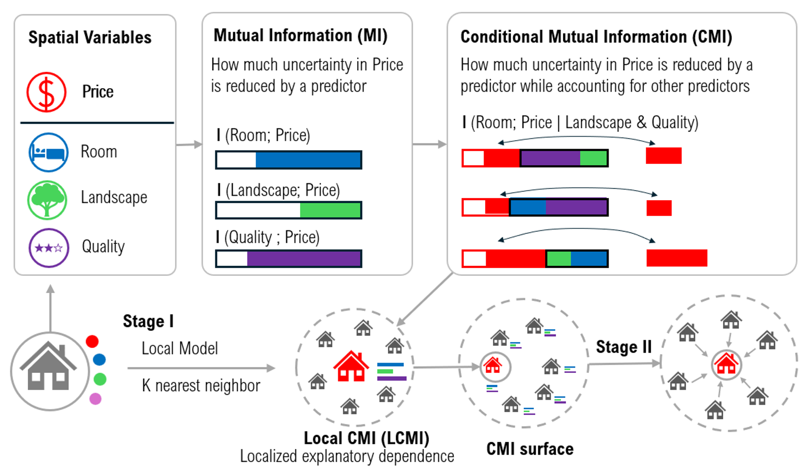
LCMI estimates how the effect of each predictor varies across space, without assuming the effect is linear. It works in two stages.
- Local dependence (stage 1). At every location, LCMI measures the conditional mutual information between each predictor and the response within a local neighbourhood. This gives an unsigned "where does x_j matter" surface.
- Spatially varying effects (stage 2). LCMI then fits a varying-coefficient model
y = b0(s) + Σj bj(s) · gj(xj).- Each
gjis a learned nonlinear transform. - Each
bj(s)is a smooth coefficient surface (penalised splines). It is reported on an interpretable scale and with a well-defined sign.
- Each
Installation
pip install geocmi
The PyPI distribution is called geocmi; the module is imported as lcmi:
from lcmi import CMI, CMIc
From source (this repository):
pip install git+https://github.com/UrbanGISer/LCMI.git
Dependencies: numpy, pandas, scipy, scikit-learn, matplotlib, joblib.
Quick start
from lcmi import CMI

model = CMI(df, u="lon", v="lat", y="y", xlist=["x1", "x2", "x3"]).fit()

model.summary()               # R² of both stages, selected k / bandwidth
model.coef_table()            # summary of the coefficient surfaces
model.plot_coefficients()     # maps of the spatially varying effects
model.plot_transforms()       # learned shapes g_j(x_j)
model.plot_pdp()              # partial-dependence decomposition (stage 1)

out = model.df_out            # your data + all LCMI columns
y_new = model.predict(new_df) # predict at new locations / predictor values
Outputs (model.df_out)
| column | meaning |
|---|---|
{x}_esd |
Spatially varying effect of x: change in y per 1 SD of the learned transform g(x). Signed, comparable across variables. Use this for maps. |
{x}_lin |
Linear-equivalent local slope dy/dx. Comparable to GWR coefficients for monotone, roughly linear effects. |
{x}_vc |
Raw multiplier b(s) of g(x). |
{x}_lws |
Stage-1 local conditional mutual information (dependence strength, unsigned). |
vc_intercept, y_pred_vc |
Intercept surface and fitted values (stage 2). |
y_pred |
Stage-1 fitted values. |
Categorical predictors. Variables listed in categorical= are one-hot encoded whenever they act as conditioning covariates. Their local information {x}_lws uses a label-free discrete–continuous estimator (Ross 2014), and their stage-2 transform is a learned category-effect profile, so results do not depend on how categories are coded. For a categorical x, b(s) > 0 means the local ranking of categories matches the overall profile, and b(s) < 0 means it is reversed. {x}_lin is not defined (NaN).
Reading signs. A coefficient b(s) > 0 means the local effect has the shape shown by plot_transforms(); b(s) < 0 means the mirror image. Each g(x) is oriented to increase with x, or, for U-shaped effects, to be high at the extremes.
Categorical data
| outcome | predictors | use |
|---|---|---|
| continuous | numeric and/or categorical | CMI(..., categorical=[...]) → signed effect maps {x}_esd |
| nominal (classes) | categorical and/or continuous | CMIc (module lcmi_c) → local (conditional) mutual information maps |
from lcmi import CMIc, quantile_codes

df["edu_q5"] = quantile_codes(df["edu"], 5)            # optional: coarse classes for a numeric variable
m = CMIc(df, u="lon", v="lat", y="vote_class",
         xlist=["edu_q5", "black_q5", "income"],
         categorical=["edu_q5", "black_q5"], bw=440)
m.fit(condition="auto")                                # or {x: [columns]}; None = pairwise only
m.summary()                                            # mean MI / CMI, ranking, reliability check
m.plot_maps(kind="cmi")                                # {x}_mi, {x}_cmi (+ _smooth) in m.df_out
How the estimators work:
- Nominal x vs nominal y. Debiased local plug-in MI: Miller–Madow corrected tables minus a permutation null, so the result is essentially unbiased in small windows.
- Continuous x vs nominal y. Discrete–continuous MI (Ross 2014) on x adjusted for the other predictors, with nominal ones one-hot encoded.
All of these are invariant to category labels.
- Conditioning.
condition=gives the local conditional MI Σ_z p(z) I(x; y | z), which separates a predictor's own information from information shared with an associated predictor. - Reliability check. The
retention_checkcolumn re-computes the estimate with a shuffled z. Values well below 0.8 mean the local strata are too sparse; use coarser classes or a largerbw. - Helper functions.
local_mi_nominal,local_mi_mixed,onehot,conditioning_matrix,cramers_v,quantile_codes.
Common options
CMI(df, u, v, y, xlist,
    k_candidates=[4, 6, 8, 10, 12],  # KSG neighbours searched in stage 1
    bw_candidates=None,              # stage-1 window sizes (None = automatic)
    n_jobs=-1,
    verbose=True,
    categorical=["land_use"],        # nominal predictors (unordered categories)
    wls=False)                       # also run the original kernel-WLS stage 2 (*_wls)

model.fit()                          # automatic k / bandwidth search
model.fit(k=8, bw=200)               # fixed values (int, or dict per variable)
model.fit_vc(n_basis=16)             # refit stage 2 with a finer spline basis
model.predict(new_df, return_components=True)   # coefficients + y at new rows
model.result.meta                    # r2, r2_vc, edf_vc, lam_vc, k_per_var, bw_per_var, ...
Examples
notebooks/LCMI_examples.ipynb covers:
- Synthetic data: recovery of known spatially varying, nonlinear effects.
- King County house prices: an empirical application.
- Benchmark: comparison with GWR, MGWR, GeoShapley and XGeoML on the synthetic data. Needs
pip install mgwr geoshapley XGeoML. - Robustness: out-of-sample prediction, and data outside LCMI's model class.
notebooks/LCMI_categorical_examples.ipynb covers categorical data:
- Synthetic, categorical predictors with a continuous outcome: sign-changing category effects, label invariance.
- Synthetic, nominal outcome: the fully nominal benchmark, correlated predictors and conditioning, and a continuous predictor.
- 2016 U.S. election (3,108 counties): pairwise and conditional maps of education, Black share, Hispanic share and density for a three-class vote outcome.
The data are in data/us_election_2016_counties.csv (public GeoDa Center data).
Method
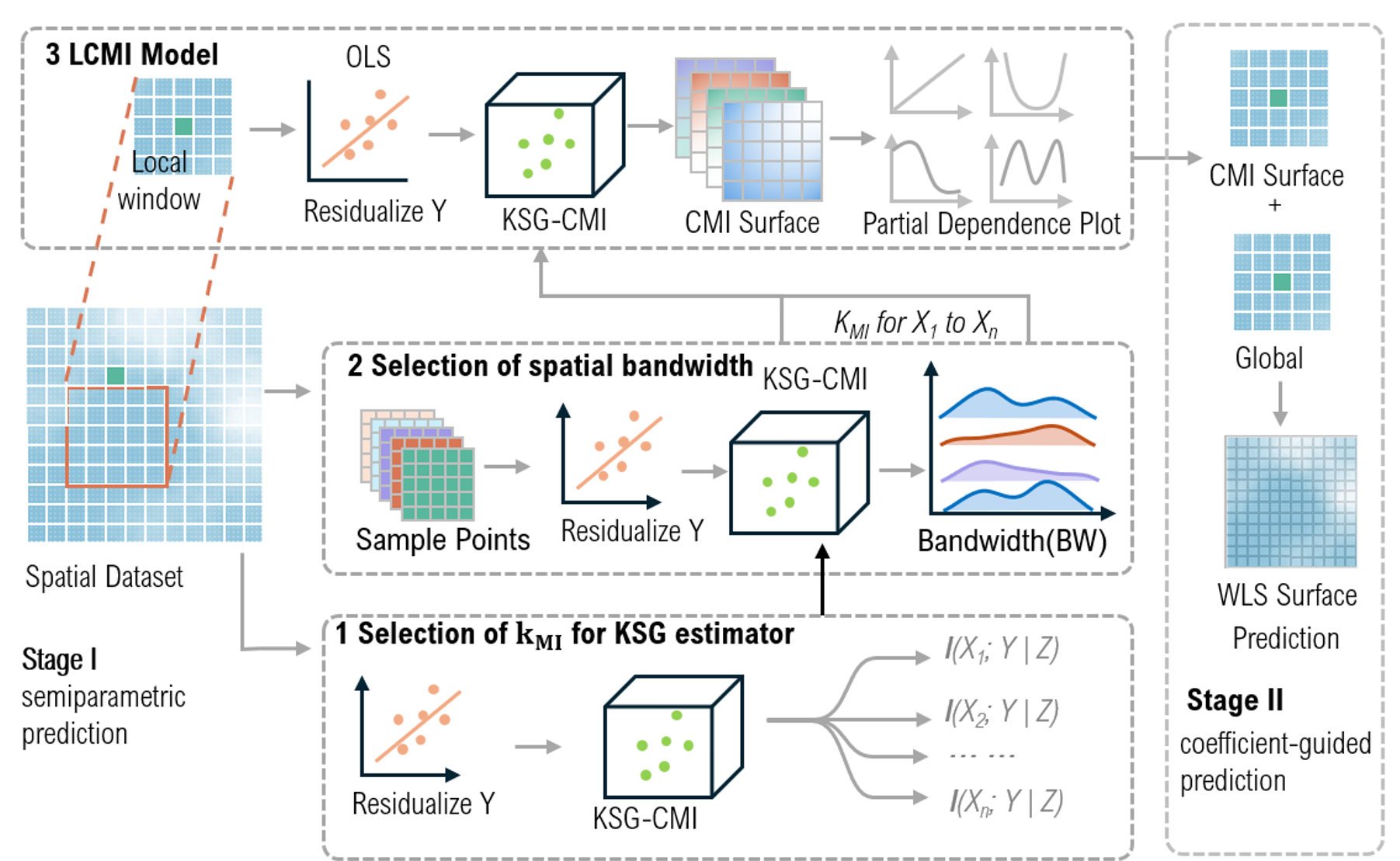
Changes relative to the code published with the paper. The paper code in lcmi-ijgis/ is kept exactly as published; the package differs as follows:
- Stage 2 is now a penalised-spline varying-coefficient model with the transforms
g_jre-estimated jointly. It replaces the kernel local WLS and gives more accurate, smoother coefficient surfaces. Signs are now absolute: the original*_wlssigns were relative to the global average effect. - Stage-1 KSG estimator uses strict neighbour counts, which reduces a downward bias in small windows.
- The original stage 2 is still available with
wls=True.
Model assumptions
- Separable effects. Stage 2 represents each effect as
bj(s) · gj(xj): one nonlinear shape whose strength and sign vary over space. When effects interact or change shape across locations, the maps give the best separable summary of them. Comparingmodel.predictout of sample with a flexible learner is a simple check. - Smooth surfaces. Coefficient surfaces are penalised splines, so very sharp spatial boundaries are smoothed. For strongly irregular study areas, a larger
n_basiscan help. - Prediction range.
predictclamps new locations to the training bounding box, and new predictor values to the training range.
Citation
Liu, L. Residualized Local Conditional Mutual Information (LCMI): A Scalable Information-Theoretic Framework for Interpretable and Nonlinear Spatially Varying Effect Modelling. International Journal of Geographical Information Science.
License
MIT
1 maintainer

Metadata
1 maintainer
Release files for geocmi 0.1.1
For a detailed explanation of source distributions (sdists) and built distributions (wheels), please see the package formats documentation.
Source distribution (sdist)
| File | Size | Uploaded | Provenance | |
|---|---|---|---|---|
| geocmi-0.1.1.tar.gz | 34.6 kB | Without provenance | Details |
Built distribution (wheel)
| File | Interpreter | ABI | Platform | Reset |
|---|---|---|---|---|
| geocmi-0.1.1-py3-none-any.whl | Python 3 | none | any | Details |
Total release size: 68.6 kB
Release files / geocmi-0.1.1.tar.gz
| Download URL | geocmi-0.1.1.tar.gz |
|---|---|
| Size | 34.6 kB |
| Tags | Source |
|
SHA-256 checksum How to use checksums |
5e532c2ac699f025b179d9e05d0429c90decc3cb72bb9b0652f8f0e595296ede
|
|
BLAKE2b-256 checksum How to use checksums |
a3f7e4f51f86b43d6d3a0abed72de2a8b63c5c6d4efd3a2133a3cf667c64213c
|
| Upload date | |
|
Uploaded using Trusted Publishing? What is trusted publishing? |
No |
| Uploaded via |
twine/6.2.0 CPython/3.9.6
|
Release files / geocmi-0.1.1-py3-none-any.whl
| Download URL | geocmi-0.1.1-py3-none-any.whl |
|---|---|
| Size | 34.0 kB |
| Tags | Python 3 |
|
SHA-256 checksum How to use checksums |
e13e46b4255f6bab4c15d8b493a1759af09116e8dca0e66c18ddd6561c115f34
|
|
BLAKE2b-256 checksum How to use checksums |
7152703fe9bfbf8e4c33c3e61de174bee5b7f93fc12aaff7b1e264972d9ef08f
|
| Upload date | |
|
Uploaded using Trusted Publishing? What is trusted publishing? |
No |
| Uploaded via |
twine/6.2.0 CPython/3.9.6
|
Security for geocmi 0.1.1
Provenance
Provenance describes where a file came from. On PyPI, provenance is shared via attestations, which provide a verifiable record of the build or publishing details. View details, limitations and caveats.
No provenance found
None of the files in this release were uploaded with provenance metadata.
A note on package security
PyPI is a repository for distributing packages, not a service for auditing them. While third-party security researchers and our staff do their best to detect and remove malicious packages, PyPI cannot guarantee the quality, security or suitability of any given package.
To learn more about protecting yourself from malicious actors, visit our package security documentation.














