
GeoEmbed
netcl-based visual feature encoders and continuous latent field projections for aerial and satellite imagery.
Core Capabilities & Metrics
- 256d L2-Normalized Vectors: Encodes aerial imagery into compact 256-dimensional unit vectors ($|z|_2 = 1.0$).
- Distance & Similarity Metrics: Because all vectors lie on the unit hypersphere, inner product directly computes cosine similarity in $[-1.0, 1.0]$:
$$S(z_1, z_2) = z_1 \cdot z_2$$
Euclidean distance is strictly monotonically related to cosine distance, making the embeddings directly compatible with standard vector indexing (FAISS, Qdrant, Milvus):
$$D_{\text{euc}}(z_1, z_2) = \sqrt{2(1 - z_1 \cdot z_2)}$$
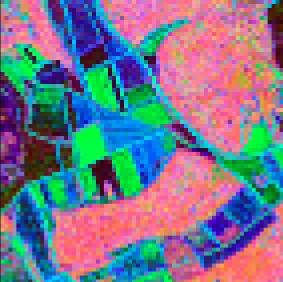
- Continuous Latent Field PCA Projection: Maps 256d embeddings into continuous 3-channel RGB color space via SVD-based PCA with robust 2%–98% percentile contrast stretching. Semantically similar landscapes receive visually neighboring hues.
- Topological & Semantic Structure: Captures road networks, parcel boundaries, forested areas, water bodies, and urban patterns without manual supervision.
- Environmental & Temporal Invariance: Robust across multi-year temporal drift, seasonal foliage variation, sun angles, and illumination shifts.
- Asynchronous Multi-Threaded Pipelining: Background CPU worker threads continuously load and preprocess tiles ahead of GPU execution (
workers=4), maintaining high inference throughput without I/O stalls.
Visual Showcase
1. Urban Center & Infrastructure Emergence (Stuttgart)
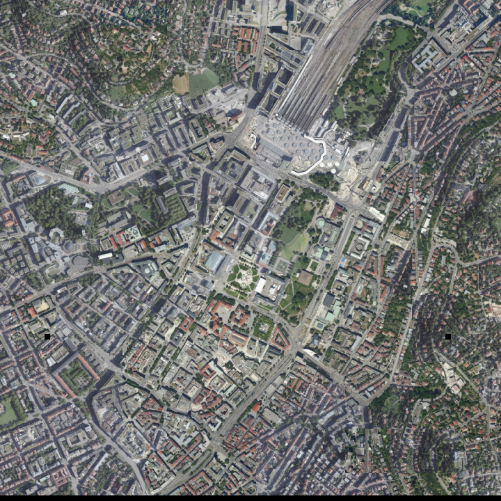
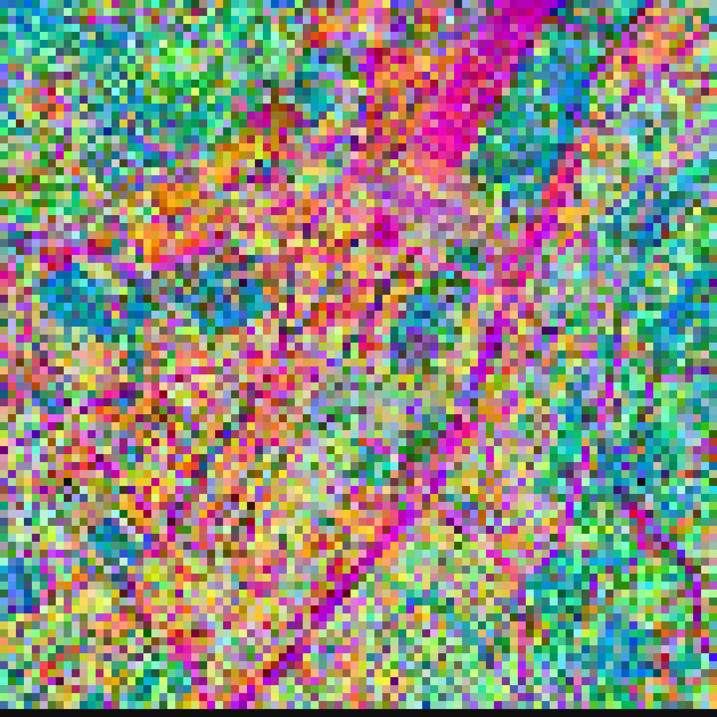
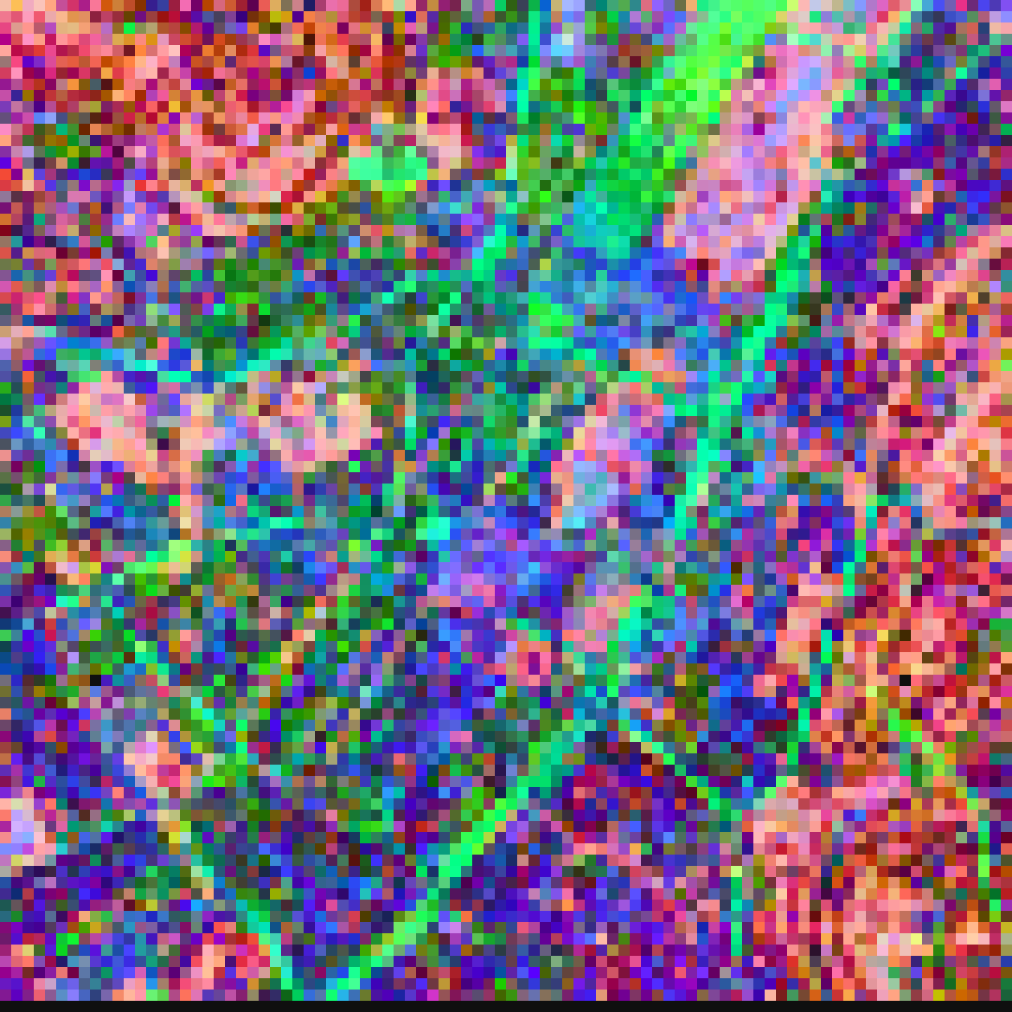
Comparing continuous latent field projections across 10,000 tiles of dense urban terrain ($z=20$, Stuttgart City Center):
| Reference Orthophoto | V3 Baseline (ResNet-18) | V11 Dual-Tower (Transformer) | V12 Refined Topology |
|---|---|---|---|
 |
 |
 |
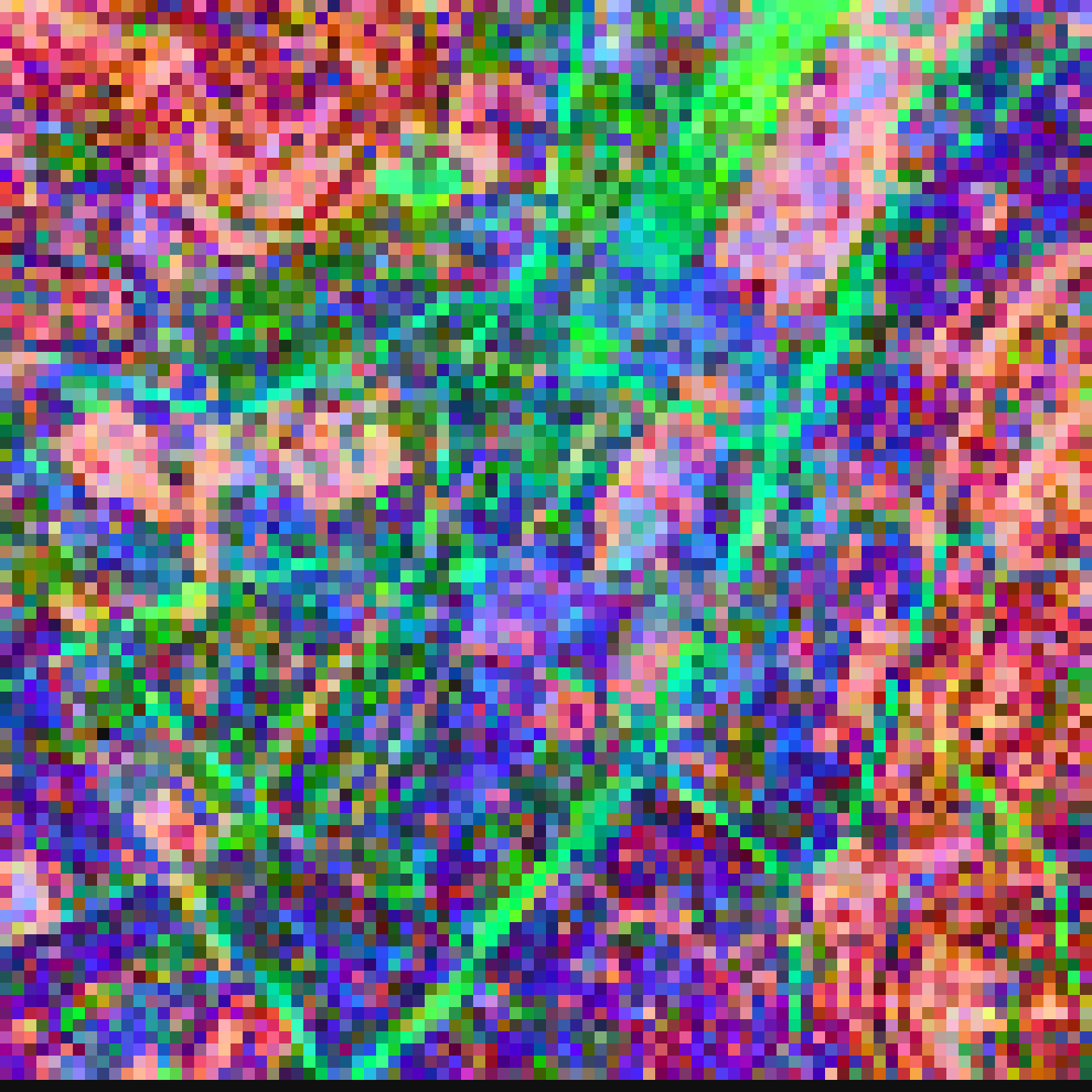 |
| True-color aerial imagery | Local texture & material variance | Relational cluster emergence | Continuous road network & urban topology |
In dense urban environments, the relational self-attention heads in V11 and V12 delineate continuous infrastructure: arterial road networks, railway corridors, and park axes emerge in vivid contrast without any manual annotations or labels.
2. Unsupervised Landscape Clustering (Rural Terrain)
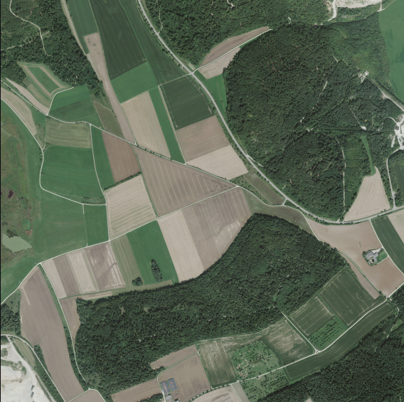
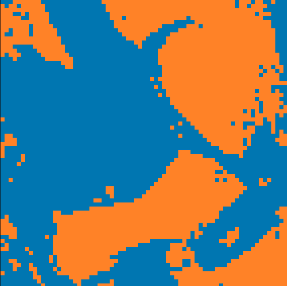
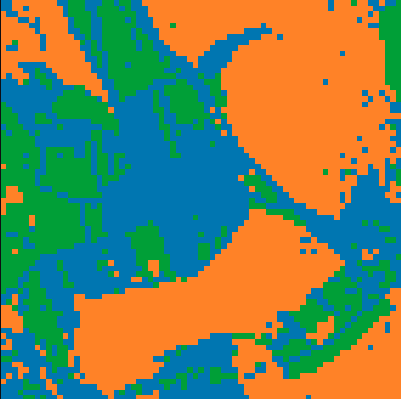
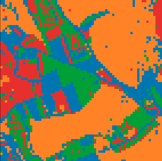
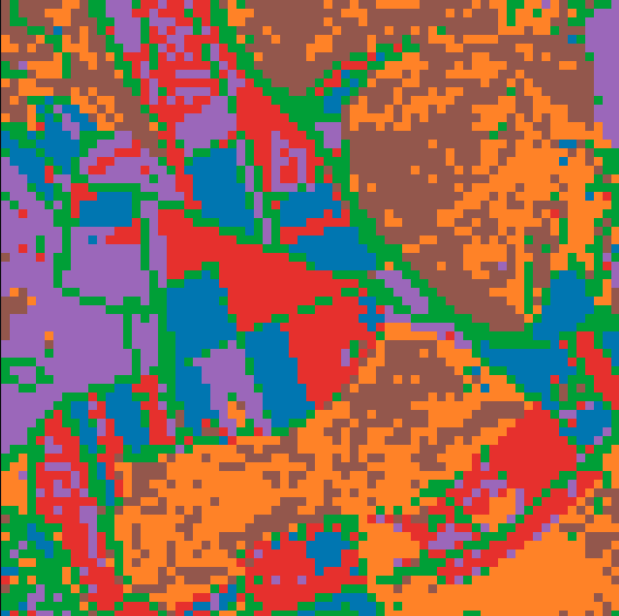
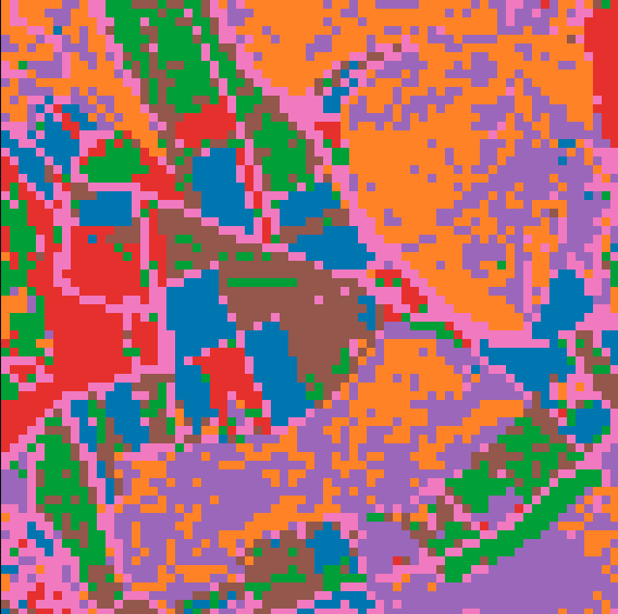
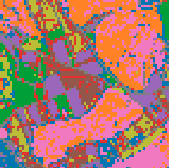
The same embeddings group natural terrain types and agricultural parcels across cluster counts $k$:
| Reference Orthophoto | Continuous Latent Field (PCA) | Low Cluster ($k=2$) |
|---|---|---|
 |
 |
 |
| Low Cluster ($k=3$) | Low Cluster ($k=4$) | Cluster Map ($k=6$) |
|---|---|---|
 |
 |
 |
| Cluster Map ($k=8$) | Cluster Map ($k=10$) | Cluster Map ($k=20$) |
|---|---|---|
 |
 |
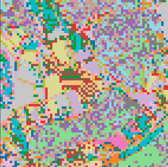 |
At low cluster counts ($k=2, 3, 4$), the latent space cleanly partitions macroscopic landscape classes (dense forest vs. open agricultural land). As $k$ increases ($k=6, 8, 10, 20$), subtle sub-structures such as access roads, parcel boundaries, and individual built structures emerge purely unsupervised.
Data source of sample orthophotos: © LGL Baden-Württemberg (www.lgl-bw.de), licensed under dl-de/by-2-0. See ATTRIBUTION.md for details.
What It Expects as Input
- Image Type: Nadir aerial and satellite imagery (orthophotos, vertical top-down view). Oblique drone or street-level photos are not supported.
- Geometry: Square image tiles (automatically resized to native resolution: $128 \times 128$ for V3, $256 \times 256$ for V11/V12).
- Format: File paths (
str/Path), raw image bytes (bytes/bytearray/ SQLite BLOBs), PILImage, or NumPy arrays. Inputs are automatically normalized to 3-channel RGB float32 in $[-1.0, 1.0]$. - Clear Preference for
z=20Web-Mercator:- Optimal Ground Scale:
z=20($\approx 0.10\text{–}0.15\text{ m/pixel}$ GSD, (\approx 38 \times 38\text{ m}) ground footprint). - Why $z=20$ is Optimal: All models show a clear empirical performance peak at $z=20$. At this ground scale, physical ground features (single building footprints, street widths, parcel borders) align directly with the receptive field of the neural network. Spatial coherence and distance-decay curves reach their maximum contrast.
- Scale Robustness across Models:
- V3: Highly sensitive to scale. Calibrated strictly for $z=20$ footprints ($\approx 38\text{ m}$). On coarser scales ($z \le 18$), an entire neighborhood block is packed into a single tile, creating high-frequency texture noise unless processed via quadtree sub-patching.
- V11 & V12: Substantially more robust against scale shifts. The dual-tower architecture and relational self-attention over the token grid preserve macro-zone clustering and spatial boundaries even across coarser scales ($z=16\text{–}19$).
- Scale Consistency Rule: Any consistent scale works, but all queries and database tiles must share the exact same ground scale. Do not mix different zoom levels within one index.
- Optimal Ground Scale:
Model Variations
| Model | Native Size | Throughput (GPU) | Architecture | Description |
|---|---|---|---|---|
V12 (Model.v12()) |
$256 \times 256$ px | ~72 tiles/s | Dual-Tower + Relational Transformer | Production default. Refined topological regularization; sharpest road network delineation. |
V11 (Model.v11()) |
$256 \times 256$ px | ~76 tiles/s | Dual-Tower + Relational Transformer | Factorized structure and fine detail towers with relational self-attention. |
V3 (Model.v3()) |
$128 \times 128$ px | ~216 tiles/s | ResNet-18 Baseline | Lightweight, fast visual encoder. Calibrated for $z=20$; high material/vegetation fidelity. |
All models output 256-dimensional unit vectors ($|z|_2 = 1.0$).
Code Examples
1. Encoding & Similarity API
from geoembed import Model

model = Model.v12(device="gpu", workers=4)

# Single tile -> np.ndarray of shape (256,)
vector = model.encode("tile.png")

# Batch encoding -> np.ndarray of shape (N, 256)
vectors = model.encode(tile_paths, batch_size=32)

# Streaming generator -> yields batches of shape (B, 256)
for batch in model.iter_encode(tile_paths, batch_size=32):
    print(batch.shape)  # (32, 256), dtype=float32

# Cosine similarity -> float in [-1.0, 1.0]
sim = model.similarity("tile_a.png", "tile_b.png")
2. Continuous Latent Field PCA Raster Map
Project tile embeddings directly into 2D continuous RGB maps with percentile contrast stretching:
# Returns PIL.Image.Image (or np.ndarray if as_image=False)
pca_map = model.render_pca_grid(
    images=tile_paths,
    coords=tile_coords,  # List of (x, y) spatial tile coordinates
    as_image=True,
)
pca_map.save("stuttgart_pca.png")
3. Multi-Scale Zoom Resampling & Super-Resolution
The models are calibrated for native $z=20$ ground footprints ($\approx 0.15\text{ m/px}$, $\approx 38\text{ m}$ per tile). When ingesting coarser imagery (e.g. $z=18$, $\approx 150\text{ m}$ footprint), evaluating full tiles directly causes scale aliasing. geoembed resolves this via quadtree sub-patching:
# Mode A: Super-Resolution (z18 input -> 16x finer z20 latent field)
# Slices each z18 tile into 16 sub-crops at native z20 footprint,
# expanding the output into a 4x4 coordinate grid.
pca_superres = model.render_pca_grid(
    images=tiles_z18,
    coords=coords_z18,
    input_zoom=18,
    target_zoom=20,
    output_zoom=20,
)

# Mode B: Noise-Free Pooled Macro Parcels (z18 -> z20 -> pooled z18)
# Evaluates sub-crops at native scale, then pools vectors back to 1 per tile.
# Eliminates high-frequency texture noise across regional maps.
pca_clean = model.render_pca_grid(
    images=tiles_z18,
    coords=coords_z18,
    input_zoom=18,
    target_zoom=20,
    output_zoom=18,
)
1 maintainer

Metadata
1 maintainer
Release files for geoembed 1.1.0
For a detailed explanation of source distributions (sdists) and built distributions (wheels), please see the package formats documentation.
Source distribution (sdist)
| File | Size | Uploaded | Provenance | |
|---|---|---|---|---|
| geoembed-1.1.0.tar.gz | 49.4 MB | Without provenance | Details |
Built distribution (wheel)
| File | Interpreter | ABI | Platform | Reset |
|---|---|---|---|---|
| geoembed-1.1.0-py3-none-any.whl | Python 3 | none | any | Details |
Total release size: 98.8 MB
Release files / geoembed-1.1.0.tar.gz
| Download URL | geoembed-1.1.0.tar.gz |
|---|---|
| Size | 49.4 MB |
| Tags | Source |
|
SHA-256 checksum How to use checksums |
014cdff2a184d9defc60e114704db3cb70b1cbf4d5661f141be4bddda848912a
|
|
BLAKE2b-256 checksum How to use checksums |
bd3122c811a8654156e97117c65d88f6be048bb3b48b8e12bb345b0f7327bb56
|
| Upload date | |
|
Uploaded using Trusted Publishing? What is trusted publishing? |
No |
| Uploaded via |
twine/6.2.0 CPython/3.12.3
|
Release files / geoembed-1.1.0-py3-none-any.whl
| Download URL | geoembed-1.1.0-py3-none-any.whl |
|---|---|
| Size | 49.4 MB |
| Tags | Python 3 |
|
SHA-256 checksum How to use checksums |
d143a03ff76e0264fd771bbb7323f10ee2e1286b6ee34d834762ea167643964a
|
|
BLAKE2b-256 checksum How to use checksums |
03447d58261505d83d5a030338d67820cd70396b1f85d50c37c4bc4ed2b8a2f4
|
| Upload date | |
|
Uploaded using Trusted Publishing? What is trusted publishing? |
No |
| Uploaded via |
twine/6.2.0 CPython/3.12.3
|
Security for geoembed 1.1.0
Provenance
Provenance describes where a file came from. On PyPI, provenance is shared via attestations, which provide a verifiable record of the build or publishing details. View details, limitations and caveats.
No provenance found
None of the files in this release were uploaded with provenance metadata.
A note on package security
PyPI is a repository for distributing packages, not a service for auditing them. While third-party security researchers and our staff do their best to detect and remove malicious packages, PyPI cannot guarantee the quality, security or suitability of any given package.
To learn more about protecting yourself from malicious actors, visit our package security documentation.














