
GeoLoupe





Explore large scientific and geospatial datasets on an interactive map: from the whole planet down to 10 m, through time, with the values one click away.
GeoLoupe puts gridded data on a web map: weather and climate reanalyses, model output, satellite images, elevation models, land cover, and station records. It reads them where they are (Zarr, NetCDF, GRIB, GeoTIFF/COG, CSV, Parquet; local or in public cloud buckets) and reads only what the screen can show. Datasets of different resolution become one seamless layer: zoomed out, you see the coarse global field; zoom in, and the fine data takes over where it exists.
Install
pip install "geoloupe[all]" # Python ≥ 3.11; or: uv tool install "geoloupe[all]"
geoloupe alone installs the core (Zarr, NetCDF); the extras add readers: remote (S3, GCS,
HTTPS), geotiff (COG), grib, stations (Parquet), vector (GeoJSON, Shapefile, …), dask
(many NetCDF files as one). all installs them all.
The geoloupe command uses the system's HTTPS certificates. In your own Python code (a notebook),
an error CERTIFICATE_VERIFY_FAILED means that Python has no certificate list: call
geoloupe.certs.use_system_certificates() before opening remote data, or set
SSL_CERT_FILE="$(python3 -m certifi)".
Try it: the gallery of open data
geoloupe gallery # → http://localhost:8000
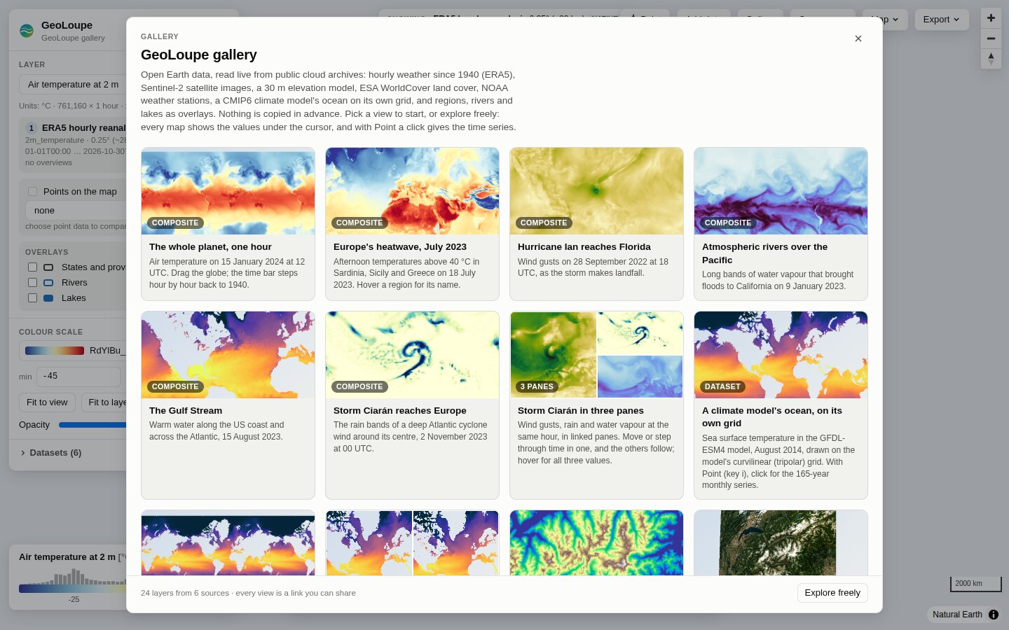
The gallery needs an internet connection and nothing else: no download in advance, no account, no key. The server starts in 10–30 s (it reads the remote metadata), and a map tile takes 0.3–1.5 s over the internet.
| Data | Source | What you can do |
|---|---|---|
| ERA5 hourly reanalysis, 0.25°, 1940 → last week (temperature, rain, water vapour, wind gusts, sea temperature) | ARCO-ERA5 Zarr on Google Cloud, 761 160 hourly steps | step hour by hour, play, compare two dates, time series of any point |
| Copernicus DEM GLO-30 (30 m), six 1° tiles in the Western Alps, over ERA5's 31 km orography | Copernicus DEM COGs on AWS | zoom from 31 km to 30 m in one layer |
| Sentinel-2 L2A, 10 m: the 10 least cloudy scenes of August 2023 over the Western Alps | a STAC search of Earth Search (Element84), COGs on AWS | one seamless mosaic in true colour, false colour (near infrared) or single bands, side by side |
| ESA WorldCover 2021, 10 m, 45–48° N, 6–9° E | ESA WorldCover COG on AWS | 11 land-cover classes with names, colours and shares of the view |
| GFDL-ESM4 climate model ocean (CMIP6 historical), monthly 1850–2014, on its native tripolar grid | Pangeo CMIP6 Zarr on Google Cloud | a curvilinear model grid drawn as it is; difference of two months 165 years apart |
| States and provinces, rivers, lakes (overlays) | Natural Earth 1:10m GeoJSON | switch on in the layer panel; hover a region for its name next to the data value |
| GHCN-Daily stations, 21 long records (Milan since 1763) | NOAA NCEI CSV files | daily max/min temperature and precipitation; with Point, click a station for its whole record |
The gallery is a normal configuration file: geoloupe gallery --show-config prints it, so you can
copy it and change it.
Your own data
No configuration is needed for a first look:
uv run geoloupe serve /path/to/data.zarr        # or .nc, .grib2, .tif, a URL
uv run geoloupe serve grid.zarr stations.csv     # several files; tables become point layers
uv run geoloupe serve grid.zarr regions.geojson  # vector files become overlays
uv run geoloupe serve s3://copernicus-dem-30m/Copernicus_DSM_COG_10_N46_00_E007_00_DEM/Copernicus_DSM_COG_10_N46_00_E007_00_DEM.tif  # public S3: no setup
uv run geoloupe serve s3://bucket/data.zarr --endpoint https://os.example.org --anon   # S3-compatible store
uv run geoloupe serve config.yaml --open-root ~/data   # "Add data" may also open local files below ~/data
uv run geoloupe info  /path/to/data.zarr        # what GeoLoupe sees: variables, grid, CRS, times
Add data in the browser. On your own machine, Add data opens any URL or S3 store (local files
only below folders given with --open-root). A server that listens on other interfaces
(--host 0.0.0.0) opens nothing unless started with --allow-open; --no-open turns it off. The
dialog remembers the data you opened before.
Data in S3 buckets: use Add data → Browse S3. List a bucket on AWS, or on any S3-compatible store
through its endpoint (MinIO, Ceph, SWITCH, Cloudflare R2, …), filter the names, and open a Zarr
store, NetCDF, GeoTIFF/COG, station table or vector file, in the active pane or in a new pane. Public
buckets need no setup. Private buckets use the credentials of the machine where GeoLoupe runs
(AWS_ACCESS_KEY_ID/AWS_SECRET_ACCESS_KEY, or a profile in ~/.aws); keys are never typed in the
browser. In a configuration file, the same access is
storage_options: {client_kwargs: {endpoint_url: https://…}, profile: work}. Private GeoTIFFs on a
non-AWS store are read by GDAL, which takes its endpoint from AWS_S3_ENDPOINT.
To combine datasets into one layer, add colour scales, or list featured views, write a small YAML file (full reference, more in examples/):
title: Elevation
datasets:
  dem:    {mosaic: [N45E006.tif, N45E007.tif, N46E006.tif, N46E007.tif], variable_name: elevation}
  global: {path: https://example.org/global-dem-1km.tif, variable_name: elevation}
layers:
  elevation:
    title: Elevation (30 m where available)
    sources:                      # the finest data wins; coarser data fills the rest
      - {dataset: dem, variable: elevation}
      - {dataset: global, variable: elevation}
views:                            # optional: the gallery start screen
  - {title: The Matterhorn, layer: elevation, center: [7.66, 45.98], zoom: 11}
On a remote machine or HPC node: run geoloupe serve config.yaml --port 8000 there and tunnel:
ssh -N -L 8000:localhost:8000 <host>. Behind JupyterHub with jupyter-server-proxy, open
…/user/<name>/proxy/8000/ (all URLs are relative).
In a notebook:
import xarray as xr, geoloupe
ds = xr.open_zarr("data.zarr")
geoloupe.show({"data": ds})           # interactive map in the cell output
Features
- Seamless multi-resolution layers. Stack sources (a 30 m DEM over a 31 km one, a regional model over a global one, a mosaic of many tiles). Per pixel, the finest source with data wins; coarser sources fill gaps and serve low zooms.
- Bounded cost at every zoom. Per tile, the engine picks the coarsest resolution level that is still
as fine as a screen pixel and never reads more than a fixed number of cells. COG overviews are used
automatically;
geoloupe overviews buildmakes overview pyramids for other formats. - Honest about what you see. A badge names the datasets, resolutions and native/overview levels on
screen; hover shows the displayed value and its source; with Point (key
i), a click gives the stored value of the native cell of every source, plus their time series. - Satellite images and STAC. RGB composites from any three bands, with stretch and gamma in the browser; automatic for 3-band images such as Sentinel-2 TCI. A STAC search (collection, area, dates, cloud cover) becomes one mosaic per band, best scene first, with scale and offset from the STAC metadata.
- Categorical data. Land cover and masks keep their class codes (never averaged): class colours and names from CF flags, a GeoTIFF palette or the config; the legend shows each class's share.
- Fast, interactive styling. Data tiles are floats; the browser colours them. Changing the colormap, range or log scale needs no new requests. 41 scientific colormaps (matplotlib, cmocean, Crameri), histogram of the values on screen, fit-to-view.
- Time and dimensions. Time slider, stepping, playback that waits for tiles, axes of a million
hourly steps; any extra dimension (pressure level, ensemble member) gets a selector. cftime
calendars (
noleap,360_day) work. - Stations and point data. Station tables (CSV, Parquet, GeoParquet; long or wide; columns detected) and CF timeSeries NetCDF are layers of their own, or are drawn over a gridded layer in its colour scale: hover shows observation, grid value and difference.
- Vector overlays. Regions, borders, rivers, catchments, tracks or sites from GeoJSON, Shapefile, GeoPackage, FlatGeobuf or GeoParquet, drawn over the data; hover shows the feature's name and attributes next to the value under the cursor.
- Split panes, like tmux. Split the map right or down (up to 6 panes), drag the dividers, and
show a different layer, time and colour scale in each pane. Panes share the camera and the time
(each can be unlinked); the hover lists every pane's value, a picked point gives every pane's time
series, and the whole layout exports as one figure. Keys:
%split right,"split down,xclose,zzoom a pane,Alt+arrows move. A linked pane can show another time: the same day, 30 years earlier (time offset). - Error maps. An error pane shows the error of one layer (P, e.g. a model) against another (T,
e.g. observations): bias, absolute, squared and relative errors, ratios, event agreement (hits,
misses, false alarms) or your own formula of P and T. It follows the panes it compares. Computed
from the native cells, not the screen pixels (errors that cancel inside a pixel still count),
with bias, MAE and RMSE (or POD, FAR, CSI) of the view, the error over time at a point, and
geoloupe errors buildfor maps that are exact at every zoom. See docs/errors.md. - Open data from S3 buckets. Add data → Browse S3 lists a bucket on AWS or any S3-compatible store (MinIO, Ceph, SWITCH, Cloudflare R2, …), shows what GeoLoupe can open, and opens it in a pane; public buckets need no setup, private ones use the server's own credentials.
- Many formats and grids. Zarr v2/v3 (sharded, consolidated or not), NetCDF 3/4 and HDF5 (also multi-file), GRIB, GeoTIFF/COG (multi-band, palettes), kerchunk/VirtualiZarr references; local or remote (HTTPS, S3, GCS). Public S3 buckets work without credentials or setup. Lat/lon grids in either longitude convention, Gaussian grids, projected CRSs (UTM, LAEA, rotated pole, …), and curvilinear grids with 2-D longitude/latitude (ocean models, WRF, CMIP6 native grids, swaths).
- Gallery and sharing. Featured views as a start screen, also with several panes; every view is a link (layout included); PNG export with title, colour bar and attribution (one pane or the whole layout); the data in view as NetCDF; time series as CSV.
- Python and Jupyter.
geoloupe.show(...)puts any xarray Dataset on the map inside a notebook. The HTTP API (OpenAPI docs at/api/docs) works from any language.
Screenshots
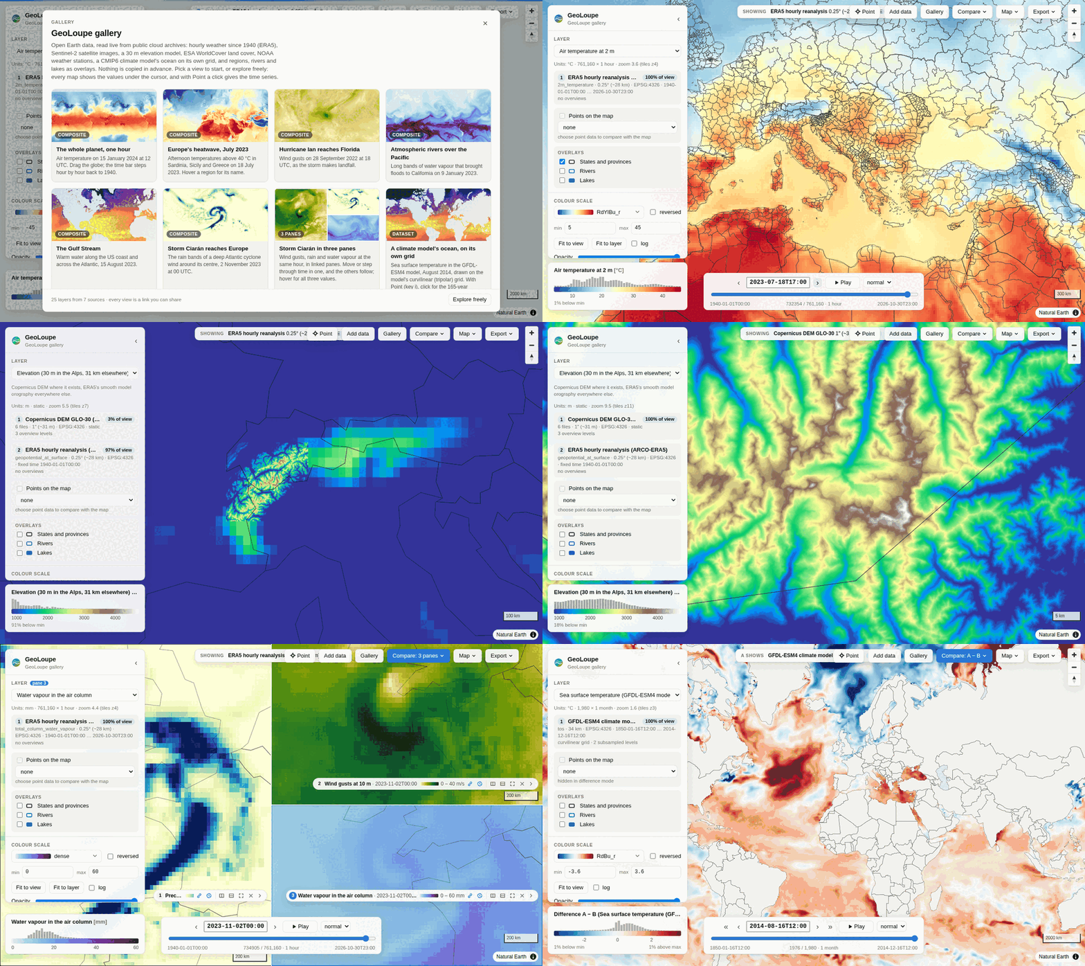
All from geoloupe gallery:
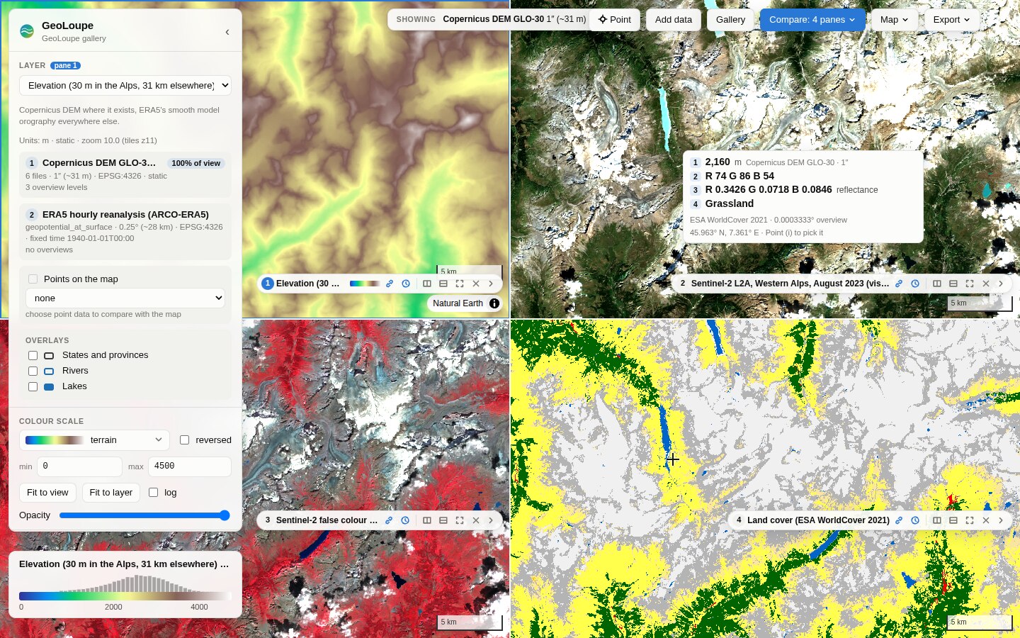 Four linked panes over the Western Alps. Elevation, Sentinel-2 in true and false colour, and land cover; the hover lists all four values, and the other panes mark the point. |
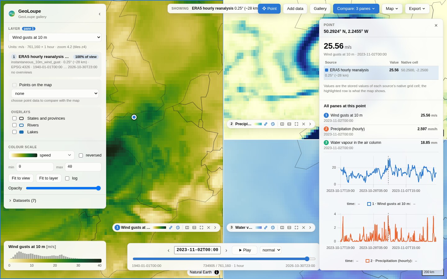 Storm Ciarán in three panes. Wind gusts, rain and water vapour at the same hour; a picked point (Point) shows every pane's value and its time series. |
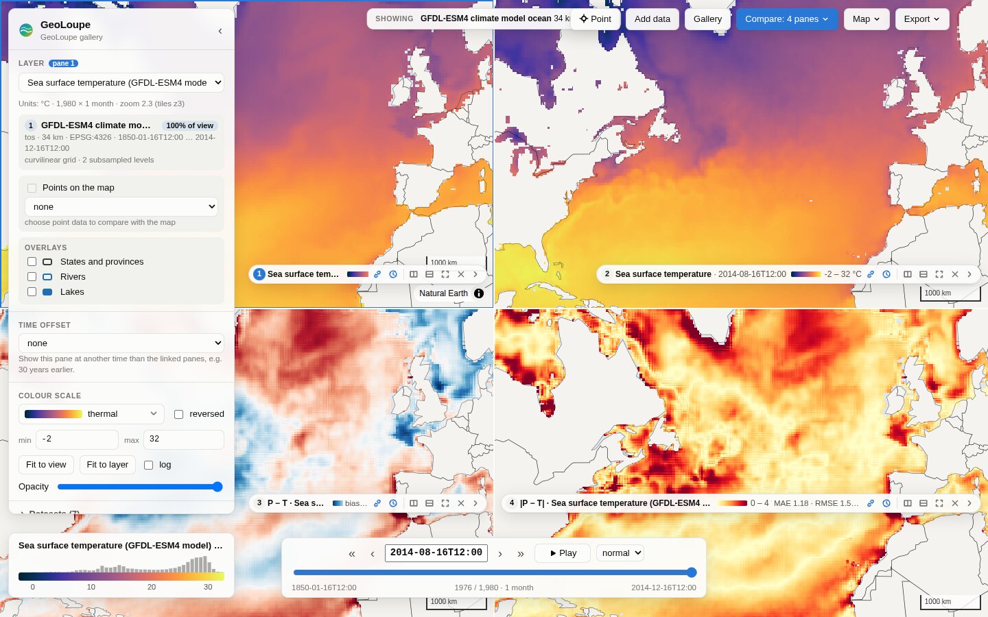 How far is a climate model from the reanalysis? The GFDL-ESM4 model (P) and ERA5 (T), with the bias P − T and the absolute error |P − T| from the native cells; the boxes give bias, MAE and RMSE of the view. |
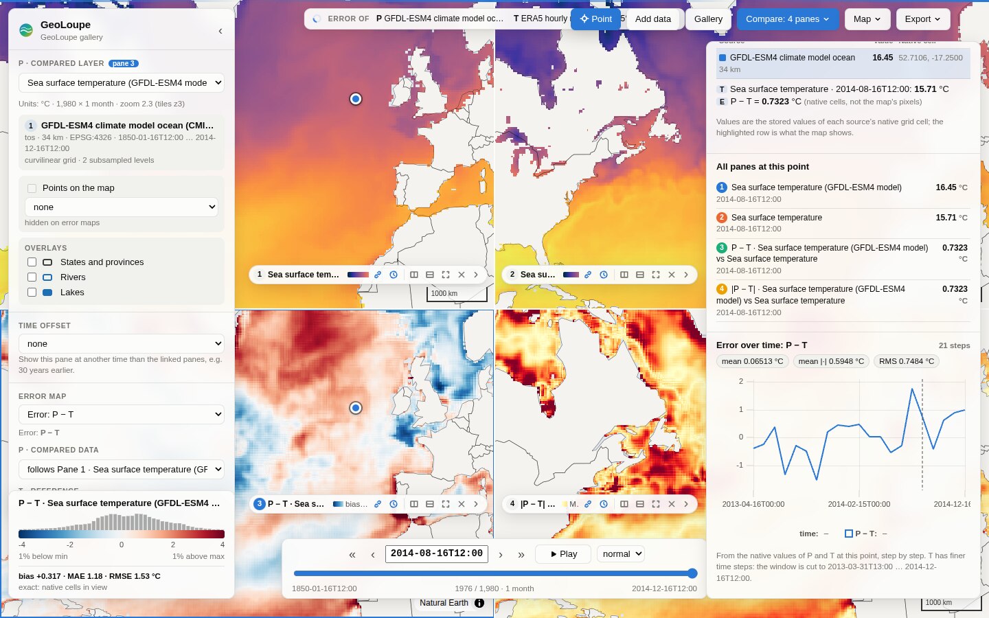 The error at a point, over time. P, T and P − T from their native values, the other panes' values, and the error month by month with its mean and RMS. |
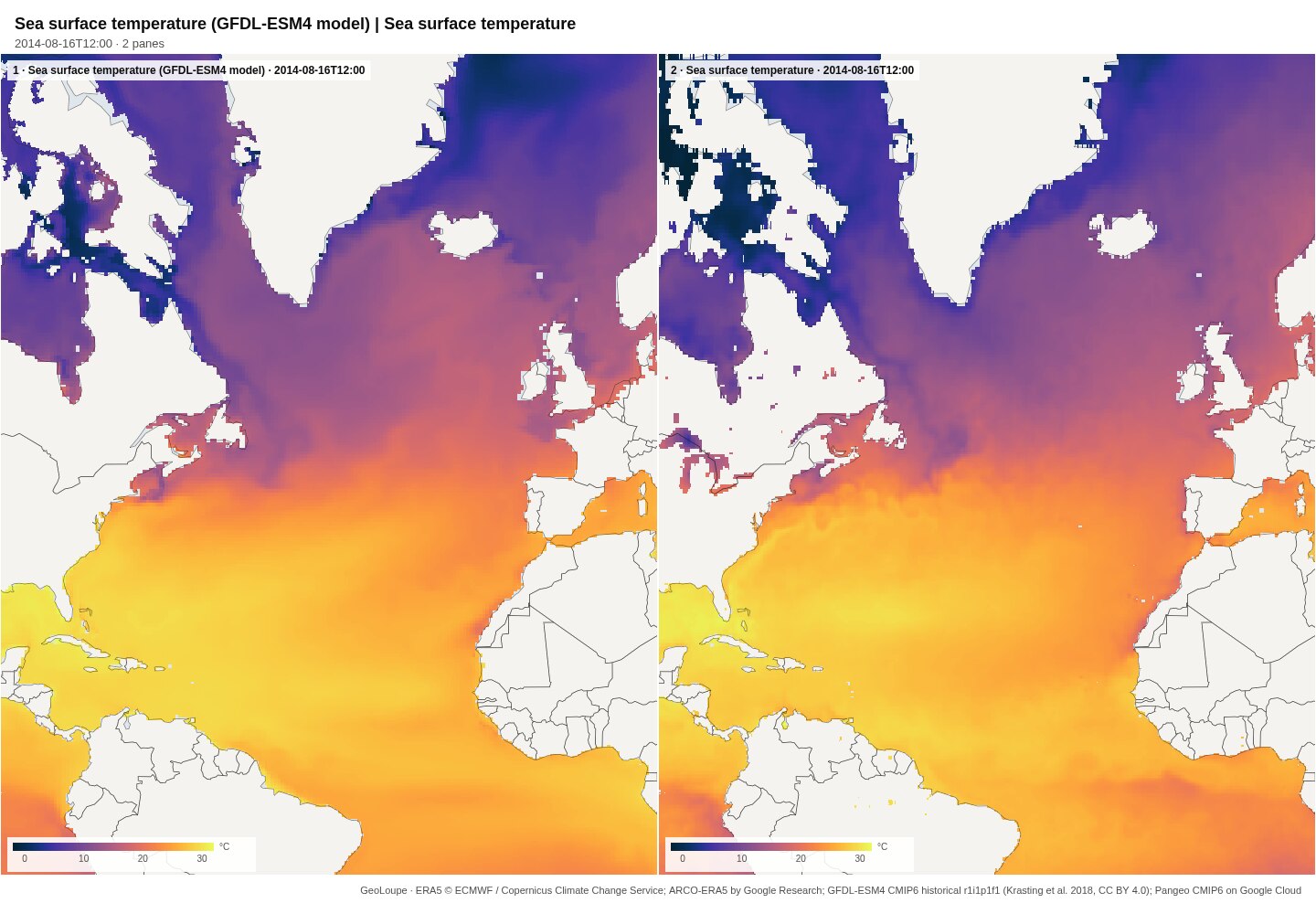 The whole layout as one figure (Export). The GFDL-ESM4 climate model next to ERA5, August 2014, each pane with its label and colour bar. |
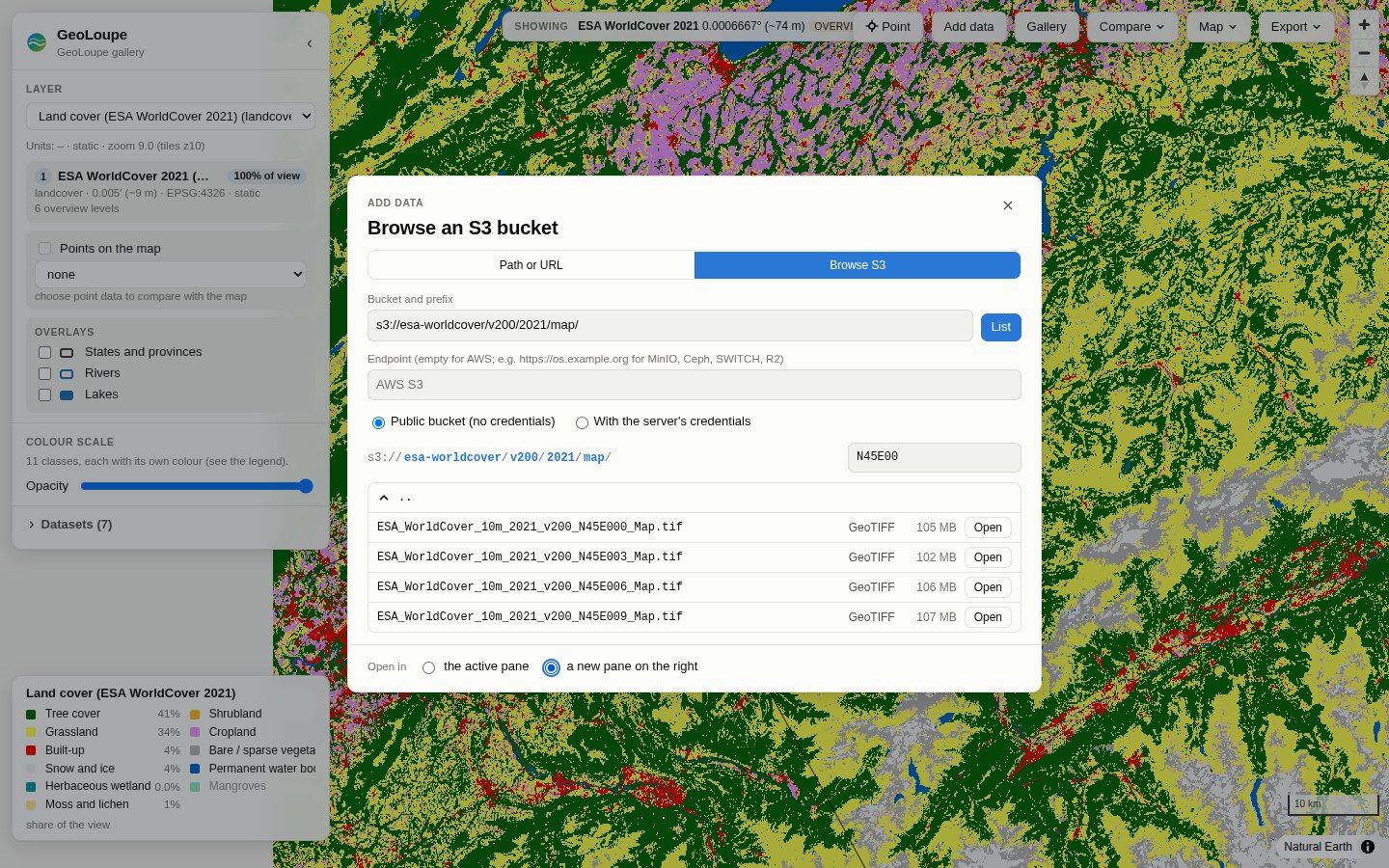 Add data → Browse S3. A public AWS bucket, filtered by name; each entry says what it is, and opens in the active pane or a new one. |
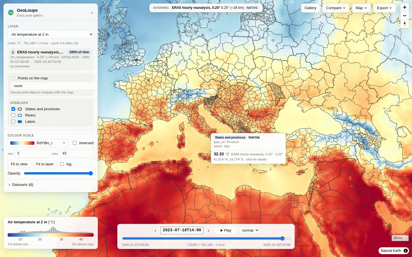 Europe's heatwave, 18 July 2023, 14 UTC. ERA5 2 m temperature, one of 761 160 hourly steps read straight from Google Cloud, with provinces as an overlay: the hover shows the region and the value. |
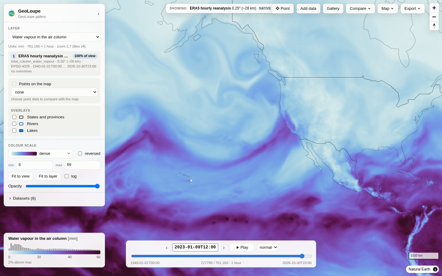 An atmospheric river reaches California, 9 January 2023. Total column water vapour. |
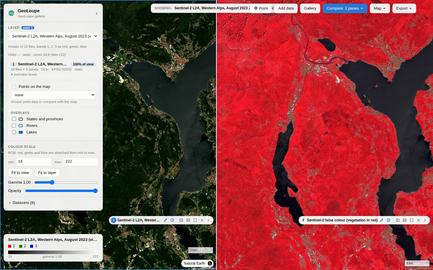 Sentinel-2, true vs false colour. Two linked panes of a STAC mosaic; the false-colour pane (near infrared as red) has its own colour scale. |
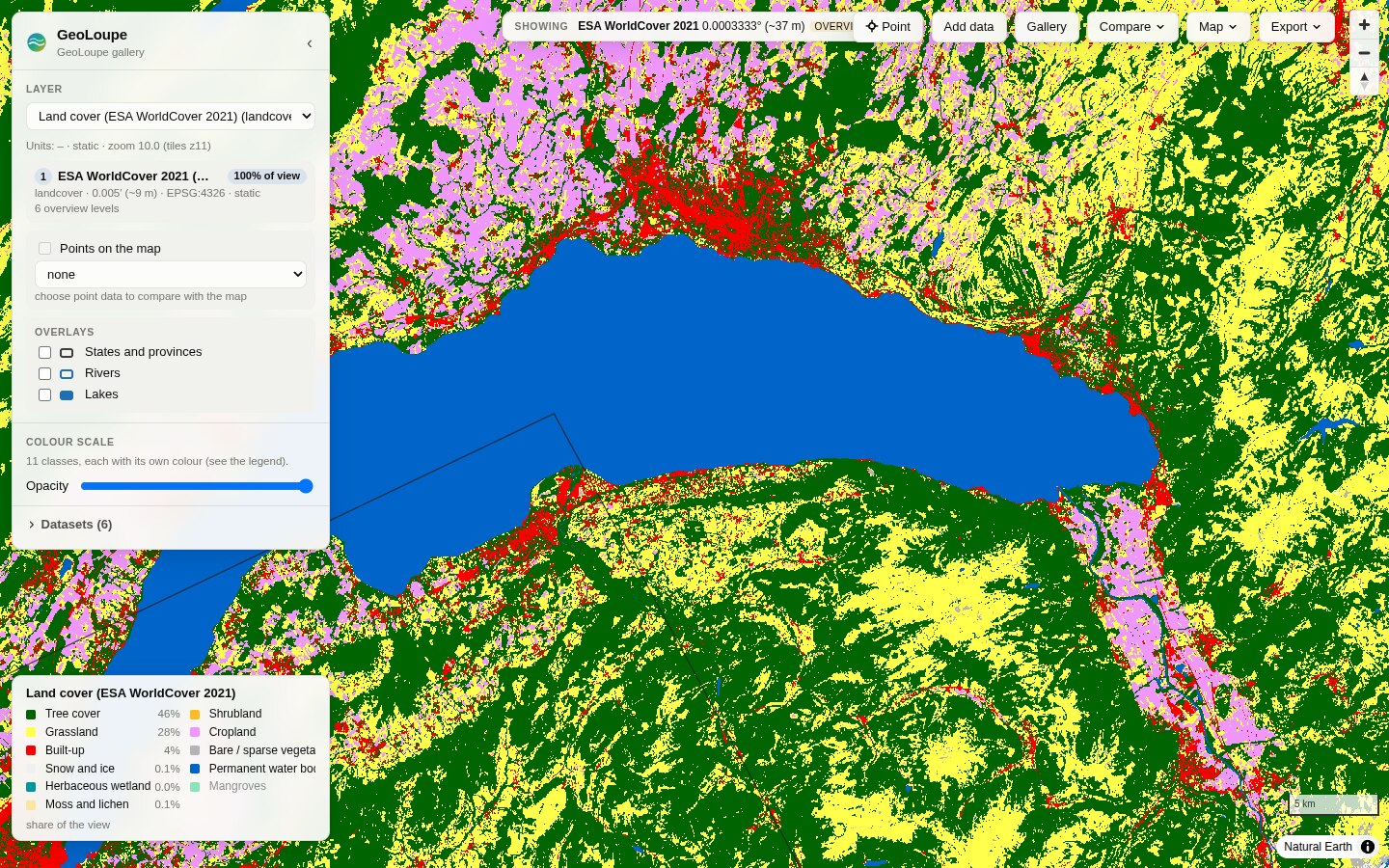 ESA WorldCover around Lake Geneva. Class colours from the file's palette, names from the config, shares of the view in the legend. |
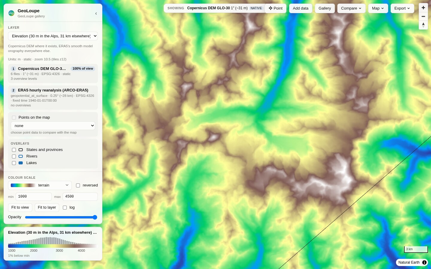 The Matterhorn in the Copernicus DEM (30 m). Six 1° tiles form one layer, with ERA5's orography outside them. |
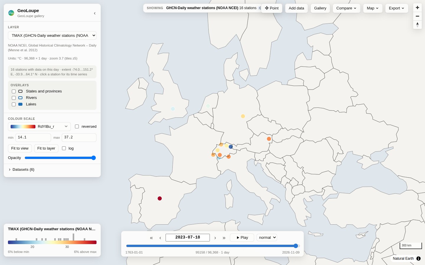 GHCN-Daily stations, 18 July 2023. With Point, click one for its whole daily record. |
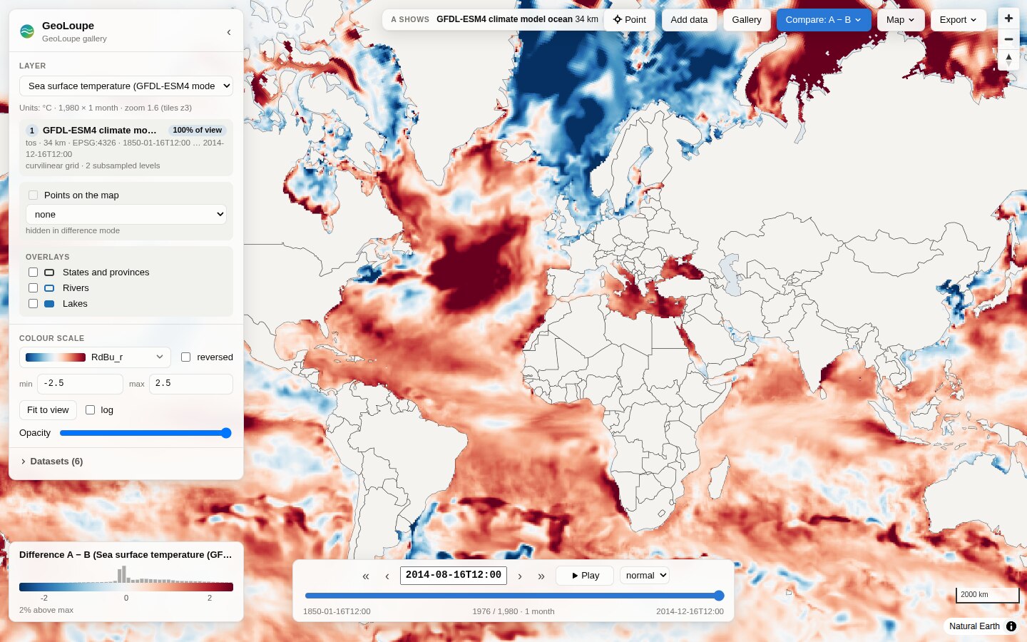 165 years of ocean warming in a climate model. GFDL-ESM4 (CMIP6) sea surface temperature on its own curvilinear (tripolar) grid, August 2014 minus August 1850. |
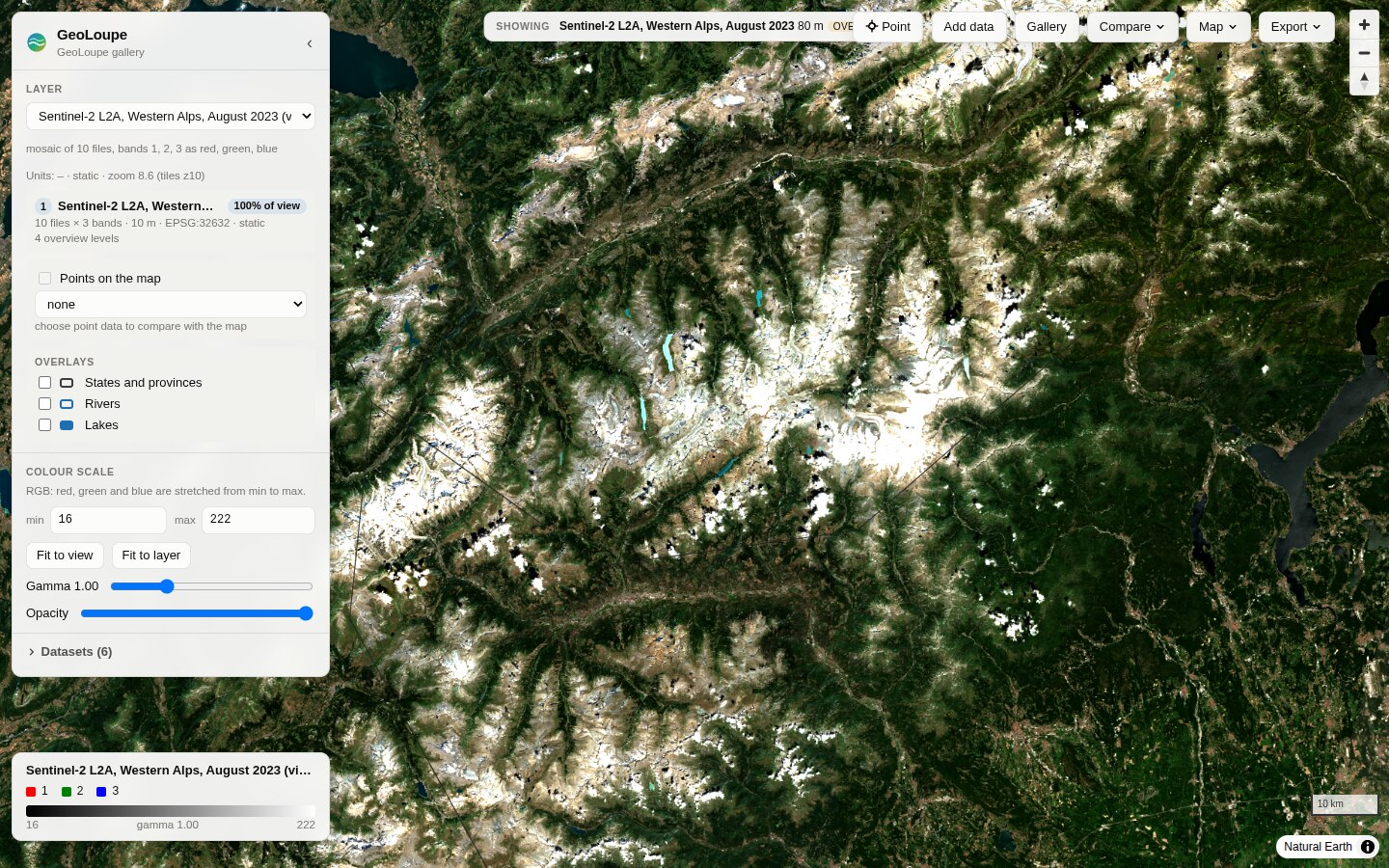 The Western Alps from space. The 10 least cloudy Sentinel-2 scenes of August 2023, found with a STAC search and shown as one seamless mosaic. |
The synthetic demo (geoloupe demo-data demo && geoloupe serve demo/demo.yaml) works offline
and shows compositing, pressure levels and a LAEA-projected grid (images).
How it works
Browser: React UI + MapLibre GL JS ── geoloupe:// protocol: fetch float tile → colour → ImageBitmap
            ▲  float32 data tiles (+ which source filled each pixel)
Server:  FastAPI ── TileEngine: per tile and source: level choice → read budget → block mean → composite
            ▲  lazy window reads (xarray, GDAL)
Data:    Zarr / NetCDF / GRIB / GeoTIFF / CSV / Parquet, local or object storage  +  optional overviews
Read ARCHITECTURE.md for the design, the data flow and the alternatives considered, docs/research.md for the survey of existing tools (TiTiler, xpublish-tiles, zarr-layer, OpenLayers GeoZarr, GeoZarr conventions, …), and docs/decisions.md for the decision log.
Status and limitations
GeoLoupe 0.3 is young but complete enough for daily use (see ROADMAP.md):
- Grids: rectilinear and curvilinear. Unstructured meshes (UGRID, HEALPix, ICON) are not supported
yet. Curvilinear grids show the nearest cell (no averaging) and get coarser levels by subsampling;
geoloupe overviews builddoes not support them yet. - Tiles: Web Mercator (plus MapLibre's globe view). Polar regions beyond ±85° are not shown.
- On-the-fly aggregation is an unweighted mean of the cells whose centres fall in a pixel; projected grids use nearest neighbour (build overviews for means).
- Point time series read one chunk per time step. Data chunked for maps (one time step per chunk) makes long series slow (seconds per year of daily data).
- Remote data is as fast as the network: the first view of a remote COG or Zarr store takes a few seconds; later reads use GDAL's and the server's caches.
- No authentication or multi-user features; bind to localhost or use an authenticating proxy. This
matters most for Add data (remote URLs, on by default on localhost;
--open-root), which lets any visitor make the server read URLs (and list S3 buckets, with the server's credentials) or local files below the given folders. - GeoLoupe always runs a server; there is no browser-only mode for static GeoZarr pyramids yet.
Private GeoTIFFs on a non-AWS S3 store need
AWS_S3_ENDPOINT(GDAL reads them). - Error maps are exact from the native cells only within a read budget (for 1 km data: from about
zoom 5); wider views need
geoloupe errors build. Error maps of curvilinear or composite layers cannot be precomputed yet. - Data binned along lines (transects, fjord or river profiles) cannot be shown on the map yet.
Contributing
Contributions are welcome: bug reports, data that does not open, ideas, code and docs. Start with CONTRIBUTING.md (development setup, tests, conventions) and the open items in ROADMAP.md. In short:
git clone https://github.com/salmanmohebi/geoloupe.git && cd geoloupe
uv sync --all-extras && uv run pytest              # Python
cd frontend && npm ci && npm test && npm run dev   # web client (with the API on port 8000)
scripts/ci_local.sh                                # all CI checks on a fresh clone, before a PR
Please report security problems privately (SECURITY.md). Everyone taking part follows the code of conduct. Changes are listed in CHANGELOG.md.
Citing
If GeoLoupe helps your research, please cite it (CITATION.cff; GitHub's "Cite this repository" button gives BibTeX and APA). Each release is archived on Zenodo: 10.5281/zenodo.24156973 cites the latest version; the Zenodo page lists the DOI of each version.
License and data credits
Apache License 2.0. Colormaps: matplotlib (BSD-compatible / CC0), cmocean (MIT), Scientific colour maps by F. Crameri (MIT). Country borders: Natural Earth (public domain).
Gallery data: ERA5 © ECMWF / Copernicus Climate Change Service, ARCO-ERA5 by Google Research; Copernicus DEM GLO-30 © DLR e.V. and Airbus Defence and Space GmbH, provided under COPERNICUS by the EU and ESA; Sentinel-2 contains modified Copernicus Sentinel data 2023, COGs by Element84; ESA WorldCover 2021 © ESA WorldCover project (CC BY 4.0); GHCN-Daily, NOAA NCEI (Menne et al. 2012); Natural Earth (public domain).
1 maintainer

Metadata
1 maintainer
Release files for geoloupe 0.3.0
For a detailed explanation of source distributions (sdists) and built distributions (wheels), please see the package formats documentation.
Source distribution (sdist)
| File | Size | Uploaded | Provenance | Actions |
|---|---|---|---|---|
| geoloupe-0.3.0.tar.gz | 1.4 MB | With provenance | Details for geoloupe-0.3.0.tar.gz |
Built distribution (wheel)
| File | Interpreter | ABI | Platform | Actions Reset |
|---|---|---|---|---|
| geoloupe-0.3.0-py3-none-any.whl | Python 3 | none | any | Details for geoloupe-0.3.0-py3-none-any.whl |
Total release size: 2.3 MB
Release files / geoloupe-0.3.0.tar.gz
| Download URL | geoloupe-0.3.0.tar.gz |
|---|---|
| Size | 1.4 MB |
| Tags | Source |
|
SHA-256 checksum How to use checksums |
0c3f966953a3e22dd3cd9b77ffde4d5f15c7cad778ee377a1fe4cbcff411e97f
|
|
BLAKE2b-256 checksum How to use checksums |
ddcd8465f9a1ae21f36b70405a0b4c9582936bdf69a75596884c9eb0c0298c62
|
| Upload date | |
|
Uploaded using Trusted Publishing? What is trusted publishing? |
Yes |
| Uploaded via |
twine/7.0.0 CPython/3.13.16
|
Provenance
Provenance describes where a file came from. On PyPI, provenance is shared via attestations, which provide a verifiable record of the build or publishing details. View details, limitations and caveats.


PyPI Publish Attestation
PyPI verified that this artifact, at this checksum, originated from the publisher listed below.
Signed by GitHub Actions, verified by PyPI on Nov 13, 2026.
Transparency logRelease files / geoloupe-0.3.0-py3-none-any.whl
| Download URL | geoloupe-0.3.0-py3-none-any.whl |
|---|---|
| Size | 836.1 kB |
| Tags | Python 3 |
|
SHA-256 checksum How to use checksums |
4127b33b292fd0f649b71766fc1dff20b08bc080f2a1dc7437724eb92f2c6146
|
|
BLAKE2b-256 checksum How to use checksums |
9ef4bda43362d81e22d42c59e4c273938fa4681a02b583edadf9229d5a218994
|
| Upload date | |
|
Uploaded using Trusted Publishing? What is trusted publishing? |
Yes |
| Uploaded via |
twine/7.0.0 CPython/3.13.16
|
Provenance
Provenance describes where a file came from. On PyPI, provenance is shared via attestations, which provide a verifiable record of the build or publishing details. View details, limitations and caveats.
PyPI Publish Attestation
PyPI verified that this artifact, at this checksum, originated from the publisher listed below.
Signed by GitHub Actions, verified by PyPI on Nov 13, 2026.
Transparency logSecurity for geoloupe 0.3.0
Provenance
Provenance describes where a file came from. On PyPI, provenance is shared via attestations, which provide a verifiable record of the build or publishing details. View details, limitations and caveats.
Full provenance
Both files in this release have been uploaded with provenance metadata.
Attestation for geoloupe-0.3.0.tar.gz
PyPI Publish Attestation
PyPI verified that this artifact, at this checksum, originated from the publisher listed below.
Signed by GitHub Actions, verified by PyPI on Nov 13, 2026.
Transparency logA note on package security
PyPI is a repository for distributing packages, not a service for auditing them. While third-party security researchers and our staff do their best to detect and remove malicious packages, PyPI cannot guarantee the quality, security or suitability of any given package.
To learn more about protecting yourself from malicious actors, visit our package security documentation.














