
GeoSWE
Geophysical Shallow-Water Engine
A GPU finite-volume solver for the full 2D shallow-water equations,
from a 3 m coastal county to the conterminous United States on one multi-GPU node.






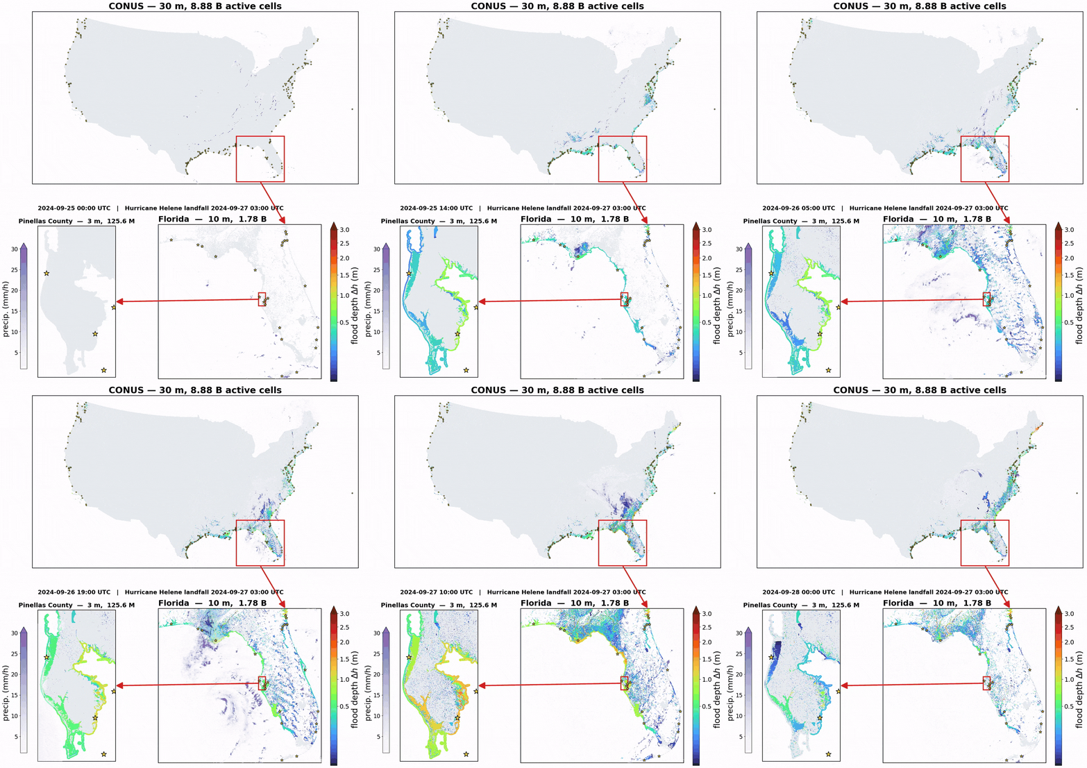
Above: 72 hours of Hurricane Helene (September 2024) simulated by the same code on three nested domains: MRMS rainfall in purple, flood depth in color, and the NOAA CO-OPS tide gauges that drive the coastal boundary as stars. Full-resolution video (MP4).
GeoSWE solves the nonlinear shallow-water equations with a well-balanced HLLC
finite-volume scheme, Manning friction, wetting and drying, rainfall, and an
observation-driven coastal stage boundary. Its distinguishing feature is a
compressed active-cell mesh: the cells that matter (land plus a nearshore
band) are packed into flat arrays before the run, so memory and work scale
with the flooded landscape rather than its bounding rectangle. The same
finite-volume kernel runs on the dense grid and on the compressed mesh: at a fixed
state the two give bit-identical residuals, and full runs agree to fp32 round-off at
the wet/dry front. It runs on NVIDIA and AMD GPUs through CuPy, scales across
GPUs with mpi4py, and falls back to NumPy on the CPU for prototyping and CI.
Highlights
| Continental domains on one node | A 72-hour Hurricane Helene scenario over CONUS at 30 m (8.88 billion active cells, 207-gauge coastal boundary) runs on eight H100 GPUs in 10.8 h; Florida at 10 m (1.78 billion active cells) on four GPUs in 9.5 h. |
| Fastest and leanest in a four-code benchmark | On a 214-million-cell county case against TRITON, SynxFlow, and SERGHEI, GeoSWE's active-cell configuration has the lowest wall time and GPU memory at every GPU count: 3.5 to 3.9 times faster and 1.5 to 1.9 times leaner than the nearest peer, with pairwise CSI near 0.99. |
| Compression costs no steps and little depth | On the standing-tide case, dense and compressed runs take identical step counts (16,051). With every cell active, which isolates the storage layout, depths agree to 0.05 cm RMSE (CSI 1.000); with the terrain-selected active set, the configuration whose speedup is quoted above, to 1.36 cm (0.02 cm on the rain-driven variant). |
| Near-ideal scaling | 99.5 % weak-scaling efficiency at 16 H100 GPUs (10.24 billion cells) and 98.8 % at 32 Blackwell MIG slices across two nodes (20.48 billion cells). |
| Thin-film accuracy | On a steady rained slope with a high-accuracy reference solution, GeoSWE stays within 1 % of the reference film depth, where TRITON and SERGHEI depart by tens of percent. SynxFlow matches it to about 1 %, which is the point: it shares the surface-reconstruction bed treatment. |
The application runs are computational demonstrations under stated, uncalibrated settings, not validated flood hindcasts.
How it compares
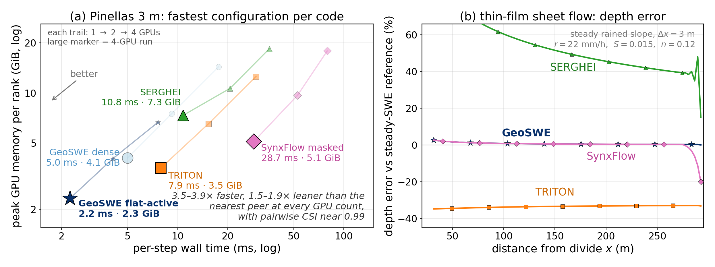
(a) Per-step wall time against peak GPU memory per rank for each code's fastest configuration on the 3 m Pinellas County benchmark (1, 2, and 4 GPUs; large marker = 4 GPUs). (b) Depth error against the steady shallow-water reference on a uniformly rained slope.
Comparison codes as benchmarked: TRITON (commit ec35bc4), SERGHEI (commit 39a10f2), and SynxFlow 1.0.2; all four in fp32 at CFL 0.5, first-order well-balanced schemes, same H100 node, identical inputs. The wet/dry floor is the one setting not held common: GeoSWE runs at 1e-6 m, SERGHEI's dryDepth was raised from 1 mm to 5 mm to stop a time-step collapse, and TRITON ran at its best-matched hextra = 1e-2. Builds, decks, and patches are in the paper's reproducibility appendix.
How it scales
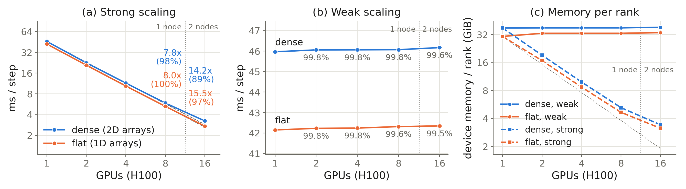
Dense and flat storage layouts on an everywhere-wet synthetic domain, 640 million cells per GPU, 1 to 16 H100 GPUs across two nodes. Strong scaling reaches 15.5x on 16 GPUs for the flat layout; weak scaling stays above 99 %.
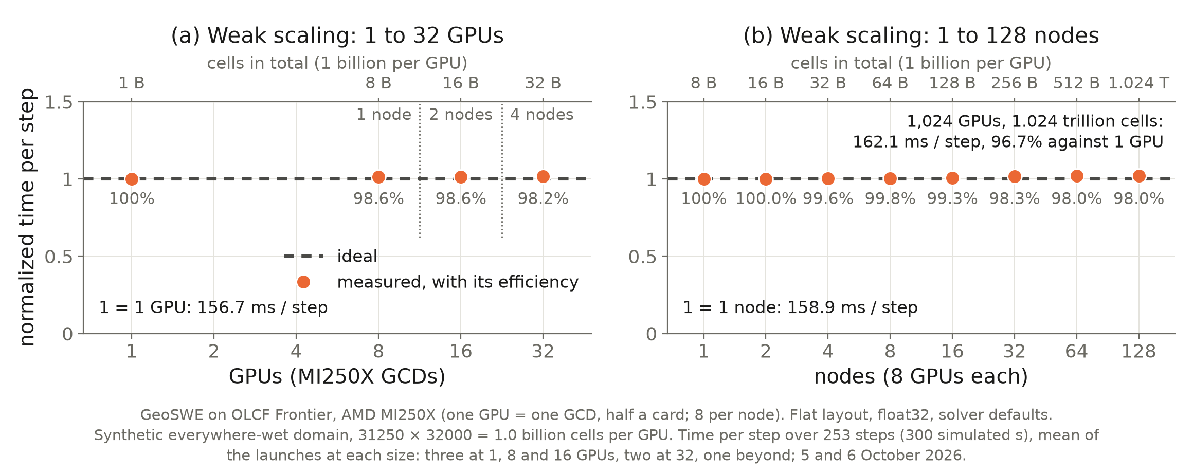
The flat layout on AMD GPUs at OLCF Frontier, one billion cells per GPU (one GCD, half of an MI250X card; eight per node): time per step divided by that of the smallest size, so ideal weak scaling is the dashed line. On 128 nodes, 1.024 trillion cells advance at 162 ms per step: 98.0 % weak-scaling efficiency against one node and 96.7 % against one GPU. A marker is the mean of up to three launches, each timed over one 40-second window; see benchmark/frontier_amd.
What is inside
- Numerics: HLLC and local Lax-Friedrichs fluxes; the Xia et al. (2017) surface-reconstruction method and Audusse hydrostatic reconstruction for exact lake-at-rest balance over arbitrary bathymetry; first-order, MUSCL, and fifth-order reconstruction; forward Euler and SSP-RK3.
- Physics: point-implicit Manning friction, wetting and drying, gridded rainfall, Green-Ampt infiltration, depth sinks, and an inverse-distance-weighted coastal stage ring driven by NOAA CO-OPS gauge records.
- Compressed active-cell mesh: static active set chosen from terrain criteria before the run,
int16neighbor offsets, a two-cell ghost halo, build-once caching, active-cell-balanced multi-GPU partitions, and checkpoint/restart. - Backends: CuPy on NVIDIA GPUs (CUDA) and AMD GPUs (ROCm), with a fused single-kernel time step;
mpi4pyfor multi-GPU runs with GPU-aware halo exchange; and a NumPy CPU fallback that runs the same scheme in float64.
Installation
# CPU only (NumPy backend): enough for the examples, tests, and docs
pip install geoswe

# GPU on CUDA 12 or CUDA 13 drivers, multi-GPU, GeoTIFF I/O, and forcing readers
# (installs one CuPy build with its CUDA headers; do not add a second CuPy build)
pip install "geoswe[gpu,mpi,io,forcings]"

# The same on an AMD GPU with ROCm 7
pip install "geoswe[gpu-rocm,mpi,io,forcings]"

# From a source checkout (needed for the examples and the bundled terrain)
git clone https://github.com/GeoSWE/geoswe.git && cd geoswe
pip install -e ".[all]"
The development version installs straight from the repository:
pip install "geoswe @ git+https://github.com/GeoSWE/geoswe.git".
See the installation page for CUDA and CuPy version notes and the conda environment, and the AMD GPUs page for ROCm.
Quick start
A storm on real terrain, from the repository root. The same script runs on the CPU (about half a minute) and on a GPU (two seconds):
import numpy as np
from geoswe import Mesh2D, Config, Solver2D, RainfallForcing

# terrain and roughness: arrays indexed [x, y], elevations in metres
case = np.load("examples/data/cookcounty_mini.npz")
win = np.s_[336:464, 336:464]                # a 1.3 km window; use np.s_[:, :] on a GPU
bed, manning = case["bed"][win], case["manning"][win]
nx, ny = bed.shape
mesh = Mesh2D(nx=nx, ny=ny, dx=float(case["dx"]), dy=float(case["dy"]))

# 75 mm/h for one hour on a dry bed; water leaves freely at the edges
rain = RainfallForcing(time_s=[0, 3600], rate_mm_h=[75, 0])
cfg = Config(friction="manning", bc_x="fall", bc_y="fall", rainfall_forcing=rain)
solver = Solver2D(mesh, cfg, np.zeros((3, nx, ny)), bed)
solver.set_manning(manning)

solver.run(t_end=2 * 3600)
peak = solver.max_depth()                    # NumPy array (nx, ny), metres
print(f"deepest water {peak.max():.2f} m; {100 * (peak > 0.05).mean():.0f}% of the area reached 5 cm")
Config() with no arguments is the production scheme of the paper (first-order
HLLC, SRM well balancing, forward Euler, CFL 0.5). The
flood tutorial explains each line and adds your own
GeoTIFF terrain, a tide or surge, and the compressed active-cell mesh.
examples/ has runnable scripts for 1D and 2D dam breaks, a
lake-at-rest check, rain on a slope, convergence order, multi-GPU scaling, a
rain-driven flood on real terrain with bundled data, and the compressed mesh on
that terrain.
Reproducing the paper
benchmark/ holds the GeoSWE-side pipeline for the paper's
benchmark cases: the four-code Pinellas County comparison, the steady sheet-flow
plane, and the synthetic scaling sweep. Each case ships the scripts that
prepare the inputs, run the simulations, and produce the reported numbers; see
benchmark/README.md for data requirements and command
sequences. The Florida and CONUS application pipelines are not part of this
release; they exercise the same solver paths as the Pinellas case.
Documentation
User guide, configuration reference, the compressed mesh, multi-GPU runs, and
the API reference: https://geoswe.readthedocs.io (or build locally with
pip install ".[docs]" && sphinx-build -b html docs docs/_build).
Citing
If you use GeoSWE, please cite it; see CITATION.cff. A paper describing the method, the cross-code benchmark, and the county-to-continent applications is in preparation.
Acknowledgments
This material is based upon work supported by the National Science Foundation under Grant No. 2325631, by a 2025 IDEaS + Cloud Hub award with support from Microsoft at the Georgia Institute of Technology, and by the U.S. Department of Energy under Contract No. DE-AC05-00OR22725 through the Genesis Mission project, in collaboration with Oak Ridge National Laboratory, the Tennessee Valley Authority, and AMD. Computing resources were provided in part by the Partnership for an Advanced Computing Environment (PACE) at Georgia Tech and by the Frontier supercomputer at the Oak Ridge Leadership Computing Facility.
License
BSD 3-Clause; see LICENSE.
1 maintainer

Metadata
1 maintainer
Release files for geoswe 1.1.1
For a detailed explanation of source distributions (sdists) and built distributions (wheels), please see the package formats documentation.
Source distribution (sdist)
| File | Size | Uploaded | |
|---|---|---|---|
| geoswe-1.1.1.tar.gz | 2.5 MB | Details |
Built distribution (wheel)
| File | Interpreter | ABI | Platform | Reset |
|---|---|---|---|---|
| geoswe-1.1.1-py3-none-any.whl | Python 3 | none | any | Details |
Total release size: 2.8 MB
Release files / geoswe-1.1.1.tar.gz
| Download URL | geoswe-1.1.1.tar.gz |
|---|---|
| Size | 2.5 MB |
| Tags | Source |
|
SHA-256 checksum How to use checksums |
a4d9bee1860e1ac85b099790a451dc5f9f2e3185c2022a7a9f744d2ca3e8992c
|
|
BLAKE2b-256 checksum How to use checksums |
2e5ef9fae15b3e71e269014c19c73d9adf58cdbb894c793bae7b4961f3699896
|
| Upload date | |
|
Uploaded using Trusted Publishing? What is trusted publishing? |
Yes |
| Uploaded via |
twine/7.0.0 CPython/3.13.14
|
Provenance
Provenance describes where a file came from. On PyPI, provenance is shared via attestations, which provide a verifiable record of the build or publishing details. View details, limitations and caveats.


PyPI Publish Attestation
PyPI verified that this artifact, at this checksum, originated from the publisher listed below.
Signed by GitHub Actions, verified by PyPI on Oct 6, 2026.
Transparency logRelease files / geoswe-1.1.1-py3-none-any.whl
| Download URL | geoswe-1.1.1-py3-none-any.whl |
|---|---|
| Size | 273.0 kB |
| Tags | Python 3 |
|
SHA-256 checksum How to use checksums |
c60fe16f07347b3e96bea6156bc798909bd89c96fae2809756811b73e5317212
|
|
BLAKE2b-256 checksum How to use checksums |
d9b49fe08c09aab9824a586fbe1499a800dae8fa4e05b00c7f654802f401b732
|
| Upload date | |
|
Uploaded using Trusted Publishing? What is trusted publishing? |
Yes |
| Uploaded via |
twine/7.0.0 CPython/3.13.14
|
Provenance
Provenance describes where a file came from. On PyPI, provenance is shared via attestations, which provide a verifiable record of the build or publishing details. View details, limitations and caveats.
PyPI Publish Attestation
PyPI verified that this artifact, at this checksum, originated from the publisher listed below.
Signed by GitHub Actions, verified by PyPI on Oct 6, 2026.
Transparency log













