
Generalized Explicit Runge-Kutta (GERK)
A package for the curious mathematicians and engineers who want to experiment the Runge-Kutta method with their own coefficients.
Motivation
I decided to create this package to give mathematicians or engineers the freedom to create and use the Runge-Kutta method of their choice, as opposed to be being locked in to whatever a package provides you.
Runge-Kutta Overview
Runge-Kutta methods aim to numerically solve ordinary differential equations of the form:
$$ \frac{\text{d}y}{\text{d}x}=f(x,y) $$
with a given initial condition $(x_0, y_0)$.
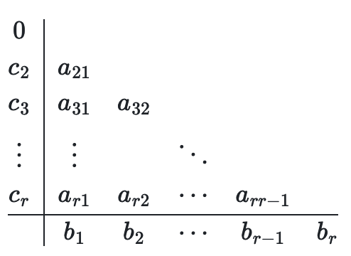
We define a member of the Runge-Kutta family with a Butcher tableau:
The above tableau is often abbreviated to
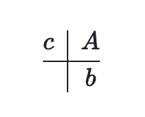
The Butcher tableau presents the categories of coefficients that will be used in our Runge-Kutta method.
The $n^\text{th}$ evaluation of the solution will be denoted as $(x_n, y_n)$. We also define $h$ as the time step i.e. the step size from the previous approximation to the next, and therefore
$$ x_{n+1} = x_{n} + h $$
Before defining $y_n$, we must familiarize ourselves with the array $k$. We define the $i^{\text{th}}$ row of $k$ at $(x_n, y_n)$ as:
$$ k_i(x_n, y_n) = f\left(x_n + c_i h, y_n + \sum_{j=1}^{i-1} a_{ij}k_j(x_n, y_n)\right) $$
where $f$ is the function defined in the differential equation above. Note the recursion in the second argument of $f$ where we sum rows preceding $k_{i}$ and apply a scale factor of $a_{ij}$.
We now have everything we need to calculate $y_{n+1}$:
$$ y_{n+1} = y_{n} + h \sum_{i=1}^{r}b_i k_{i}(x_n, y_n) $$
The idea is to calculate various slopes at point $y_n$ to ascertain a weighted of the ascent (or descent) and add it to the previous approximation.
What is Gerk?
Most packages for the Runge-Kutta method usually have the coefficients $a_{ij}$, $b_i$ and $c_i$ determined beforehand for known methods such as the Forward-Euler method, the 1/4 rule, the 3/8 rule etc, but do not allow one to customerize their own Runge-Kutta.
Gerk is an easy interface to allow the user to determine their own coefficient values for the Runge-Kutta method.
How to use Gerk
We can simply import Gerk in the following way:
from gerk import gerk
Parameters
As seen in mathematics above, there is quite a bit information required to execute the Runge-Kutta method. This has been broken down into arguments to be passed into the Gerk class:
aThe $A$ matrix in the Butcher tableau. This must be a lower triangular matrix that is formatted as a list of lists that contain floats, or integersbThe $b$ array. Must be a list of floats, decimals or integerscThe $c$ array. Must be a list of floats, decimals or integersinitialAtuplethat acts as the coordinate of the initial condition values $(x_0, y_0)$terminalThe value of $x$ for which we terminate the Runge-Kutta methodtimestepsThe number of times steps you want to apply on the from the starting point $x_0$ tofinal. Must be an integerfuncThe function expression to be numerically integratedenforce_rules(Optional) A boolean to enforce conventional Runge-Kutta rules
The function will output the time steps and approximated y values as a tuple of lists of floats.
Conditions
There is no consensus to what conditions must hold regarding the coefficients you choose for your method, however, some known Runge-Kutta methods do consistently conform to some known conditions.
These conditions are
$$\sum_{i=1}^{r}b_i=1 \ \ \ \ \sum_{i=1}^{r}b_ic_i = 1/2 \ \ \ \ \sum_{j=1}^{r}a_{ij} = c_i$$
which can be enforced by the enforce_rules parameter, which is defaulted to False.
Example
Let us numerically solve the following initial value problem:
$$ \frac{\text{d}y}{\text{d}x} = y $$
with the initial value $(0, 1)$. We want to apply a Runge-Kutta method with the following Butcher tableau:
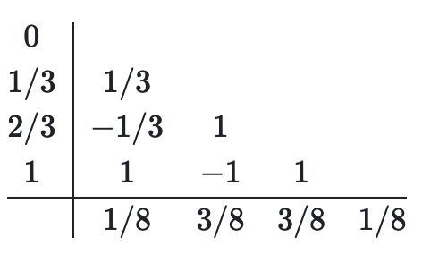
The $A$ lower triangular matrix in the Butcher tableau above can be implemented in the following way:
a = [
        [1/3],
        [-1/3, 1],
        [1, -1, 1]
]
Now for the b and c vectors:
b = [1/8, 3/8, 3/8, 1/8]

c = [0, 1/3, 2/3, 1]
Finally, we can define the function with a lambda function:
func = lambda x, y: y
Now we are ready to run gerk() and plot its output:
import matplotlib.pyplot as plt
from gerk import gerk

x, y = gerk(
        a=a,
        b=b,
        c=c,
        initial=(0, 1),
        timesteps=10000,
        terminal=1,
        func=lambda x, y: y,
    )

plt.plot(x, y, color="r")
plt.show()
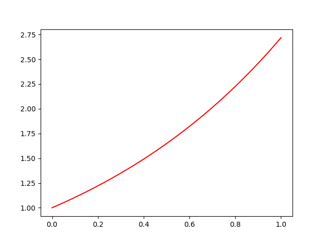
The code above yields the following graph:
Adaptive Runge-Kutta Methods
There is an alternate way to utilise the Runge-Kutta method by employing an additional distinct $b$ array. The Butcher tableau for such methods take the form:
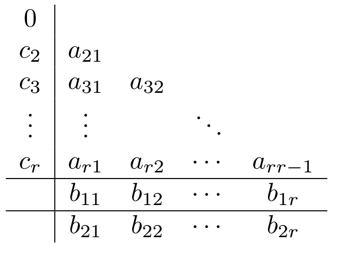
where $b_1$ and $b_2$ are the two distinct $b$ arrays.
This method is not too disimilar to the original Runge-Kutta method. We calculate the $k$'s in the same way as before, but there is an extra step when evaluating $y_{n+1}$.
Although we do calculate $y_{n+1}$ in same way outlined above, we also calculate $\gamma_{n+1}$:
$$ y_{n+1} = y_{n} + h \sum_{i=1}^{r}b_{1i}\cdot k_{i}(x_n, y_n) \ \ \ \ \ \ \ \ \ \gamma_{n+1} = y_{n} + h \sum_{i=1}^{r} b_{2i}\cdot k_{i}(x_n, y_n) $$
Note that the calculation for $\gamma$ requires the use of $y_n$ and not $\gamma_n$.
For every time step, we calculate the following error:
$$ E := \left|y_{n+1}-\gamma_{n+1}\right| $$
Now we define the tolerance, $\mathcal{E}$, which will act as the maximum acceptable value for $E$.
If $E<\mathcal{E}$, then we accept the value of $y_{n+1}$ and we increment $x_{n}$ by $h$ and start the process again for $x_{n+1}$ and $y_{n+1}$ as normal.
However, if $E\geq\mathcal{E}$, we will need to adjust the value of $h$ and redo the calculation with this renewed time step value in an attempt to satisfy the condition $E<\mathcal{E}$.
The value of $h$ will be adjusted as follows:
$$ h \rightarrow 0.9\cdot h \cdot\sqrt[n]{\frac{h}{\mathcal{E}}} $$
where $n=\min\left(p,q\right)$, where $p$ and $q$ are the orders $^1$ of $b_i$ and $b^*_i$ respectively.
$^1$ A Runge-Kutta method with matrix $a_{ij}$ and arrays $b$ and $c$ has order $p$ if
$$ \sum_{i=1}^{p}b_i = 1 \ \ \ \ \sum_{i=1}^{p}b_ic_i = 1/2 \ \ \ \ \sum_{j=1}^{p}a_{ij} = c_i \ \ \ \ $$
Adaptive Runge-Kutta example
In this example, we will try to numerically integrate
$$ \frac{\text{d}y}{\text{d}x}=-2xy $$
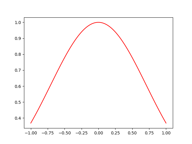
with initial conditions $(-1, e^{-1})$. Note that the exact solution is $y=e^{-x^2}$.
Here we will use the Bogacki–Shampine (BS23) method which has the following Butcher tableau:
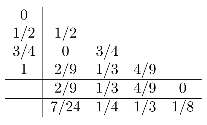
For the adaptive Runge-Kutta method, we will use adaptive_gerk(). This method's paramters vary slightly from gerk():
aThe $A$ matrix in the Butcher tableau. This must be a lower triangular matrix that is formatted as a list of lists that contain floats, or integersb_1The $b_1$ array. Must be a list of floats, decimals or integersb_2The $b_2$ array. Must be a list of floats, decimals or integerscThe $c$ array. Must be a list of floats, decimals or integersinitialAtuplethat acts as the coordinate of the initial condition values $(x_0, y_0)$terminalThe value of $x$ for which we terminate the Runge-Kutta methodtimestepsThe number of times steps you want to apply on the from the starting point $x_0$ tofinal. Must be an integerfuncThe function expression to be numerically integratedenforce_rules(Optional) A boolean to enforce conventional Runge-Kutta rules. Defaulted toFalsetolerance(Optional) A float representing the maximum threshold of the adaptive step. Defaulted to1e-4
Similar to gerk(), this function will output the time steps and approximated y values as a tuple of lists of floats.
from math import exp
import matplotlib.pyplot as plt
from gerk import adaptive_gerk

a = [
    [1/2],
    [0, 3/4],
    [2/9, 1/3, 4/9]
]
b_1 = [2/9, 1/3, 4/9, 0]
b_2 = [7/24, 1/4, 1/3, 1/8]
c = [0, 1/2, 3/4, 1]

x, y = adaptive_gerk(
        a=a,
        b_1=b_1,
        b_2=b_2,
        c=c,
        initial=(-1, exp(-1)),
        timesteps=10000,
        terminal=1,
        func=lambda x, y: -2 * x * y,
    )

plt.plot(x, y, color="r")
plt.show()
The code above yields the following graph:
In the pipeline
- To further generalise the Runge-Kutta method with an indefinite number of $b$ and $c$ arrays
- Implement Cython for faster execution times
- More descriptive error messages
- Add unit tests
- Implement Stochastic Runge-Kutta method
1 maintainer

Metadata
1 maintainer
Release files for gerk 1.0.2
For a detailed explanation of source distributions (sdists) and built distributions (wheels), please see the package formats documentation.
Source distribution (sdist)
| File | Size | Uploaded | |
|---|---|---|---|
| gerk-1.0.2.tar.gz | 6.8 kB | Details |
Built distribution (wheel)
| File | Interpreter | ABI | Platform | Reset |
|---|---|---|---|---|
| gerk-1.0.2-py3-none-any.whl | Python 3 | none | any | Details |
Total release size: 14.4 kB
Release files / gerk-1.0.2.tar.gz
| Download URL | gerk-1.0.2.tar.gz |
|---|---|
| Size | 6.8 kB |
| Tags | Source |
|
SHA-256 checksum How to use checksums |
048249fd7fc17d78187d558ec3c5bbf97ecb7508f203ac0969e000bb8978a667
|
|
BLAKE2b-256 checksum How to use checksums |
ccb98b2aca607028c252fb2b1f604a2b8f6fc9aea3f89de25f623686574b54b9
|
| Upload date | |
|
Uploaded using Trusted Publishing? What is trusted publishing? |
No |
| Uploaded via |
twine/5.1.1 CPython/3.10.6
|
Release files / gerk-1.0.2-py3-none-any.whl
| Download URL | gerk-1.0.2-py3-none-any.whl |
|---|---|
| Size | 7.6 kB |
| Tags | Python 3 |
|
SHA-256 checksum How to use checksums |
08f881af5a9ceefe51d07b8dace8a316cfcfed6c5d28ab41342e99e4f6c22e3d
|
|
BLAKE2b-256 checksum How to use checksums |
dd4754e63ce147509fac4d7cabe0f923a8caf68f910184343e47d60a5e31a74f
|
| Upload date | |
|
Uploaded using Trusted Publishing? What is trusted publishing? |
No |
| Uploaded via |
twine/5.1.1 CPython/3.10.6
|














