
Generalized Explicit Runge-Kutta (GERK)
A package for the curious mathematicians and engineers who want to experiment the Runge-Kutta method with their own coefficients.
Motivation
I decided to create this package to give mathematicians or engineers the freedom to create and use the Runge-Kutta method of their choice, as opposed to be being locked in to whatever a package provides you.
Runge-Kutta Overview
Runge-Kutta methods aim to numerically solve ordinary differential equations of the form:
$$ \frac{\text{d}y}{\text{d}x}=f(x,y) $$
with a given initial condition $(x_0, y_0)$.
We define a member of the Runge-Kutta family with a Butcher tableau:
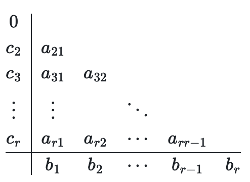
The above tableau is often abbreviated to
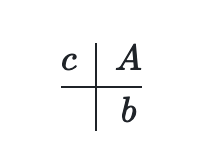
The Butcher tableau presents the categories of coefficients that will be used in our Runge-Kutta method.
The $n^\text{th}$ evaluation of the solution will be denoted as $(x_n, y_n)$. We also define $h$ as the time step i.e. the step size from the previous approximation to the next, and therefore
$$ x_{n+1} = x_{n} + h $$
Before defining $y_n$, we must familiarize ourselves with the array $k$. We define the $i^{\text{th}}$ row of $k$ at $(x_n, y_n)$ as:
$$ k_i(x_n, y_n) = f\left(x_n + c_i h, y_n + \sum_{j=1}^{i-1} a_{ij}k_j(x_n, y_n)\right) $$
where $f$ is the function defined in the differential equation above. Note the recursion in the second argument of $f$ where we sum rows preceding $k_{i}$ and apply a scale factor of $a_{ij}$.
We now have everything we need to calculate $y_{n+1}$:
$$ y_{n+1} = y_{n} + h \sum_{i=1}^{r}b_i k_{i}(x_n, y_n) $$
The idea is to calculate various slopes at point $y_n$ to ascertain a weighted of the ascent (or descent) and add it to the previous approximation.
What is Gerk?
Most packages for the Runge-Kutta method usually have the coefficients $a_{ij}$, $b_i$ and $c_i$ determined beforehand for known methods such as the Forward-Euler method, the 1/4 rule, the 3/8 rule etc, but do not allow one to customerize their own Runge-Kutta.
Gerk is an easy interface to allow the user to determine their own coefficient values for the Runge-Kutta method.
How to use Gerk
We can simply import Gerk in the following way:
from gerk import gerk
Parameters
As seen in mathematics above, there is quite a bit information required to execute the Runge-Kutta method. This has been broken down into arguments to be passed into the Gerk class:
aThe $A$ matrix in the Butcher tableau. This must be a lower triangular matrix that is formatted as a list of lists that contain floats, or integersbThe $b$ array. Must be a list of floats, decimals or integerscThe $c$ array. Must be a list of floats, decimals or integersinitialAtuplethat acts as the coordinate of the initial condition values $(x_0, y_0)$terminalThe value of $x$ for which we terminate the Runge-Kutta methodtimestepsThe number of times steps you want to apply on the from the starting point $x_0$ tofinal. Must be an integerfuncThe function expression to be numerically integratedenforce_rules(Optional) A boolean to enforce conventional Runge-Kutta rules
The function will output the time steps and approximated y values as a tuple of lists of floats.
Conditions
There is no consensus to what conditions must hold regarding the coefficients you choose for your method, however, some known Runge-Kutta methods do consistently conform to some known conditions.
These conditions are
$$\sum_{i=1}^{r}b_i=1 \ \ \ \ \sum_{i=1}^{r}b_ic_i = 1/2 \ \ \ \ \sum_{j=1}^{r}a_{ij} = c_i$$
which can be enforced by the enforce_rules parameter, which is defaulted to False.
Example
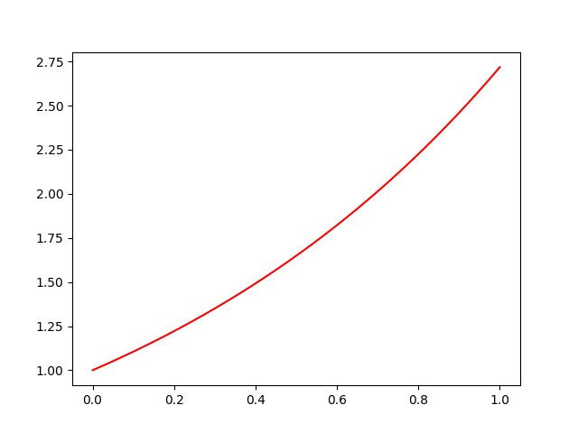
Let us numerically solve the following initial value problem:
$$ \frac{\text{d}y}{\text{d}x} = y $$
with the initial value $(0, 1)$. We want to apply a Runge-Kutta method with the following Butcher tableau:
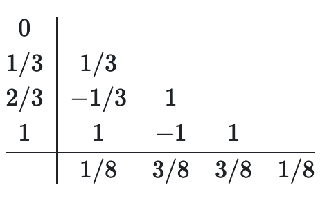
The $A$ lower triangular matrix in the Butcher tableau above can be implemented in the following way:
a = [
        [1/3],
        [-1/3, 1],
        [1, -1, 1]
]
Now for the b and c vectors:
b = [1/8, 3/8, 3/8, 1/8]

c = [0, 1/3, 2/3, 1]
Finally, we can define the function with a lambda function:
func = lambda x, y: y
Now we are ready to run gerk() and plot its output:
import matplotlib.pyplot as plt
from gerk import gerk

x, y = gerk(
        a=a,
        b=b,
        c=c,
        initial=(0, 1),
        timesteps=10000,
        terminal=1,
        func=lambda x, y: y,
    )

plt.plot(x, y, color="r")
plt.show()
The code above yields the following graph:
Adaptive Runge-Kutta Methods
There is an alternate way to utilise the Runge-Kutta method by employing an additional distinct $b$ array. The Butcher tableau for such methods take the form:
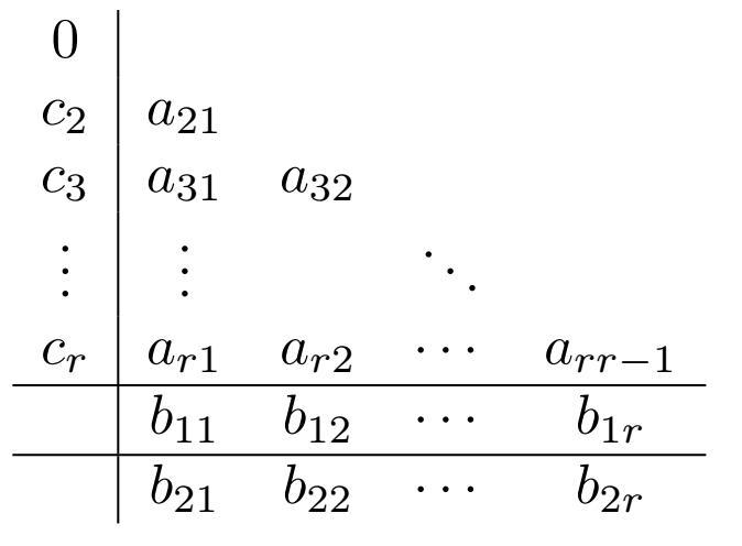
where $b_1$ and $b_2$ are the two distinct $b$ arrays.
This method is not too disimilar to the original Runge-Kutta method. We calculate the $k$'s in the same way as before, but there is an extra step when evaluating $y_{n+1}$.
Although we do calculate $y_{n+1}$ in same way outlined above, we also calculate $\gamma_{n+1}$:
$$ y_{n+1} = y_{n} + h \sum_{i=1}^{r}b_{1i}\cdot k_{i}(x_n, y_n) \ \ \ \ \ \ \ \ \ \gamma_{n+1} = y_{n} + h \sum_{i=1}^{r} b_{2i}\cdot k_{i}(x_n, y_n) $$
Note that the calculation for $\gamma$ requires the use of $y_n$ and not $\gamma_n$.
For every time step, we calculate the following error:
$$ E := \left|y_{n+1}-\gamma_{n+1}\right| $$
Now we define the tolerance, $\mathcal{E}$, which will act as the maximum acceptable value for $E$.
If $E<\mathcal{E}$, then we accept the value of $y_{n+1}$ and we increment $x_{n}$ by $h$ and start the process again for $x_{n+1}$ and $y_{n+1}$ as normal.
However, if $E\geq\mathcal{E}$, we will need to adjust the value of $h$ and redo the calculation with this renewed time step value in an attempt to satisfy the condition $E<\mathcal{E}$.
The value of $h$ will be adjusted as follows:
$$ h \rightarrow 0.9\cdot h \cdot\sqrt[n]{\frac{h}{\mathcal{E}}} $$
where $n=\min\left(p,q\right)$, where $p$ and $q$ are the orders $^1$ of $b_i$ and $b^*_i$ respectively.
$^1$ A Runge-Kutta method with matrix $a_{ij}$ and arrays $b$ and $c$ has order $p$ if
$$ \sum_{i=1}^{p}b_i = 1 \ \ \ \ \sum_{i=1}^{p}b_ic_i = 1/2 \ \ \ \ \sum_{j=1}^{p}a_{ij} = c_i \ \ \ \ $$
Adaptive Runge-Kutta example
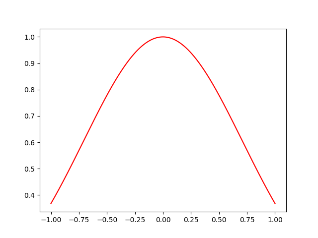
In this example, we will try to numerically integrate
$$ \frac{\text{d}y}{\text{d}x}=-2xy $$
with initial conditions $(-1, e^{-1})$. Note that the exact solution is $y=e^{-x^2}$.
Here we will use the Bogacki–Shampine (BS23) method which has the following Butcher tableau:
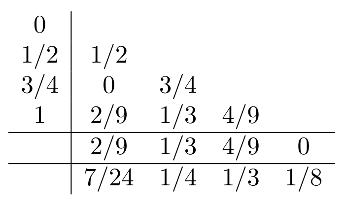
For the adaptive Runge-Kutta method, we will use adaptive_gerk(). This method's paramters vary slightly from gerk():
aThe $A$ matrix in the Butcher tableau. This must be a lower triangular matrix that is formatted as a list of lists that contain floats, or integersb_1The $b_1$ array. Must be a list of floats, decimals or integersb_2The $b_2$ array. Must be a list of floats, decimals or integerscThe $c$ array. Must be a list of floats, decimals or integersinitialAtuplethat acts as the coordinate of the initial condition values $(x_0, y_0)$terminalThe value of $x$ for which we terminate the Runge-Kutta methodtimestepsThe number of times steps you want to apply on the from the starting point $x_0$ tofinal. Must be an integerfuncThe function expression to be numerically integratedenforce_rules(Optional) A boolean to enforce conventional Runge-Kutta rules. Defaulted toFalsetolerance(Optional) A float representing the maximum threshold of the adaptive step. Defaulted to1e-4
Similar to gerk(), this function will output the time steps and approximated y values as a tuple of lists of floats.
from math import exp
import matplotlib.pyplot as plt
from gerk import adaptive_gerk

a = [
    [1/2],
    [0, 3/4],
    [2/9, 1/3, 4/9]
]
b_1 = [2/9, 1/3, 4/9, 0]
b_2 = [7/24, 1/4, 1/3, 1/8]
c = [0, 1/2, 3/4, 1]

x, y = adaptive_gerk(
        a=a,
        b_1=b_1,
        b_2=b_2,
        c=c,
        initial=(-1, exp(-1)),
        timesteps=10000,
        terminal=1,
        func=lambda x, y: -2 * x * y,
    )

plt.plot(x, y, color="r")
plt.show()
The code above yields the following graph:
In the pipeline
- To further generalise the Runge-Kutta method with an indefinite number of $b$ and $c$ arrays
- Implement Cython for faster execution times
- More descriptive error messages
- Add unit tests
- Implement Stochastic Runge-Kutta method
1 maintainer

Metadata
1 maintainer
Release files for gerk 1.0.2
For a detailed explanation of source distributions (sdists) and built distributions (wheels), please see the package formats documentation.
Source distribution (sdist)
| File | Size | Uploaded | Provenance | |
|---|---|---|---|---|
| gerk-1.0.2.tar.gz | 6.8 kB | Without provenance | Details |
Built distribution (wheel)
| File | Interpreter | ABI | Platform | Reset |
|---|---|---|---|---|
| gerk-1.0.2-py3-none-any.whl | Python 3 | none | any | Details |
Total release size: 14.4 kB
Release files / gerk-1.0.2.tar.gz
| Download URL | gerk-1.0.2.tar.gz |
|---|---|
| Size | 6.8 kB |
| Tags | Source |
|
SHA-256 checksum How to use checksums |
048249fd7fc17d78187d558ec3c5bbf97ecb7508f203ac0969e000bb8978a667
|
|
BLAKE2b-256 checksum How to use checksums |
ccb98b2aca607028c252fb2b1f604a2b8f6fc9aea3f89de25f623686574b54b9
|
| Upload date | |
|
Uploaded using Trusted Publishing? What is trusted publishing? |
No |
| Uploaded via |
twine/5.1.1 CPython/3.10.6
|
Release files / gerk-1.0.2-py3-none-any.whl
| Download URL | gerk-1.0.2-py3-none-any.whl |
|---|---|
| Size | 7.6 kB |
| Tags | Python 3 |
|
SHA-256 checksum How to use checksums |
08f881af5a9ceefe51d07b8dace8a316cfcfed6c5d28ab41342e99e4f6c22e3d
|
|
BLAKE2b-256 checksum How to use checksums |
dd4754e63ce147509fac4d7cabe0f923a8caf68f910184343e47d60a5e31a74f
|
| Upload date | |
|
Uploaded using Trusted Publishing? What is trusted publishing? |
No |
| Uploaded via |
twine/5.1.1 CPython/3.10.6
|
Security for gerk 1.0.2
Provenance
Provenance describes where a file came from. On PyPI, provenance is shared via attestations, which provide a verifiable record of the build or publishing details. View details, limitations and caveats.
No provenance found
None of the files in this release were uploaded with provenance metadata.
A note on package security
PyPI is a repository for distributing packages, not a service for auditing them. While third-party security researchers and our staff do their best to detect and remove malicious packages, PyPI cannot guarantee the quality, security or suitability of any given package.
To learn more about protecting yourself from malicious actors, visit our package security documentation.














