

ggrust




The Grammar of Graphics, written in Rust, used from Python.
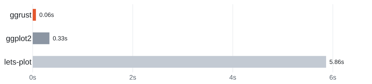
Median time to render one of 11 everyday plots with 1M rows, as SVG and PNG (benchmarks).
ggrust is a plotting library with a Lets-Plot compatible Python API. Plots are built the familiar ggplot way, layer by layer with +, while the stats, scales, layout and rendering all run in Rust.
It was started for Cellestial, which needed a maintained backend for its Lets-Plot based API.
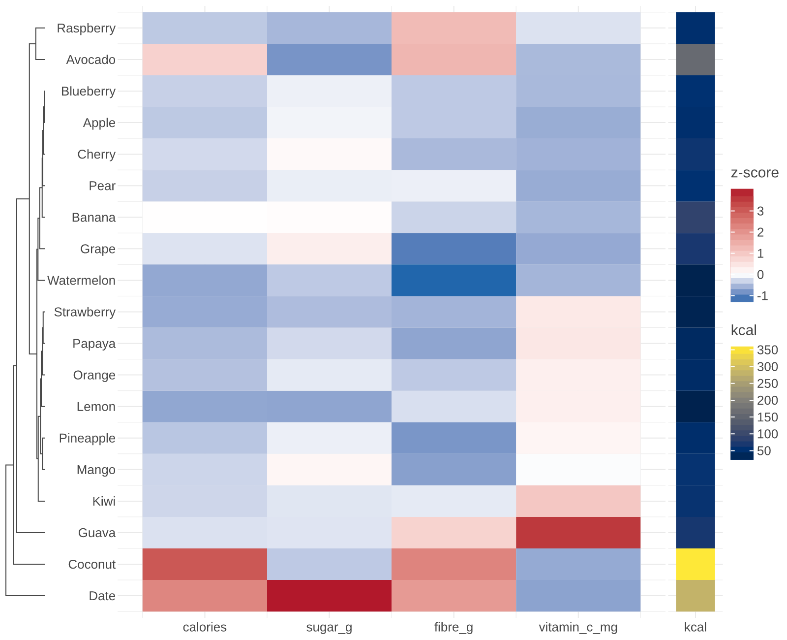
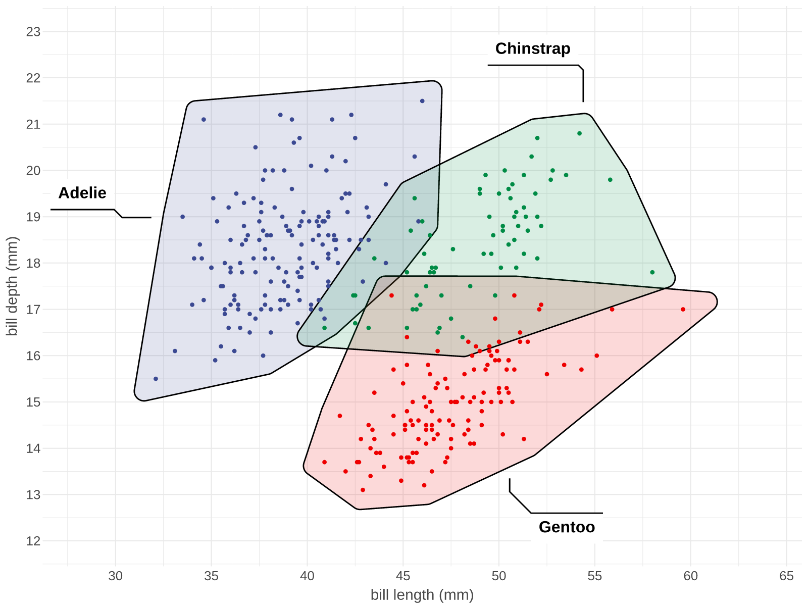
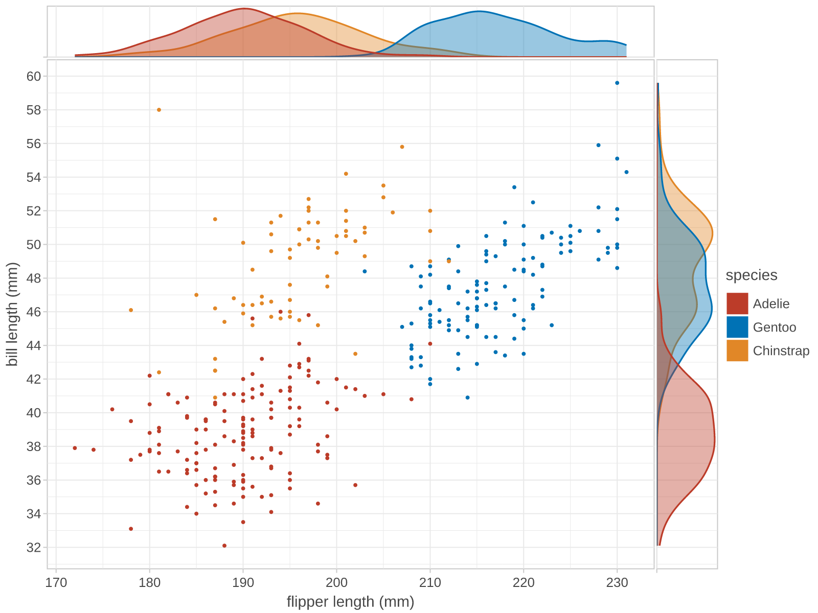
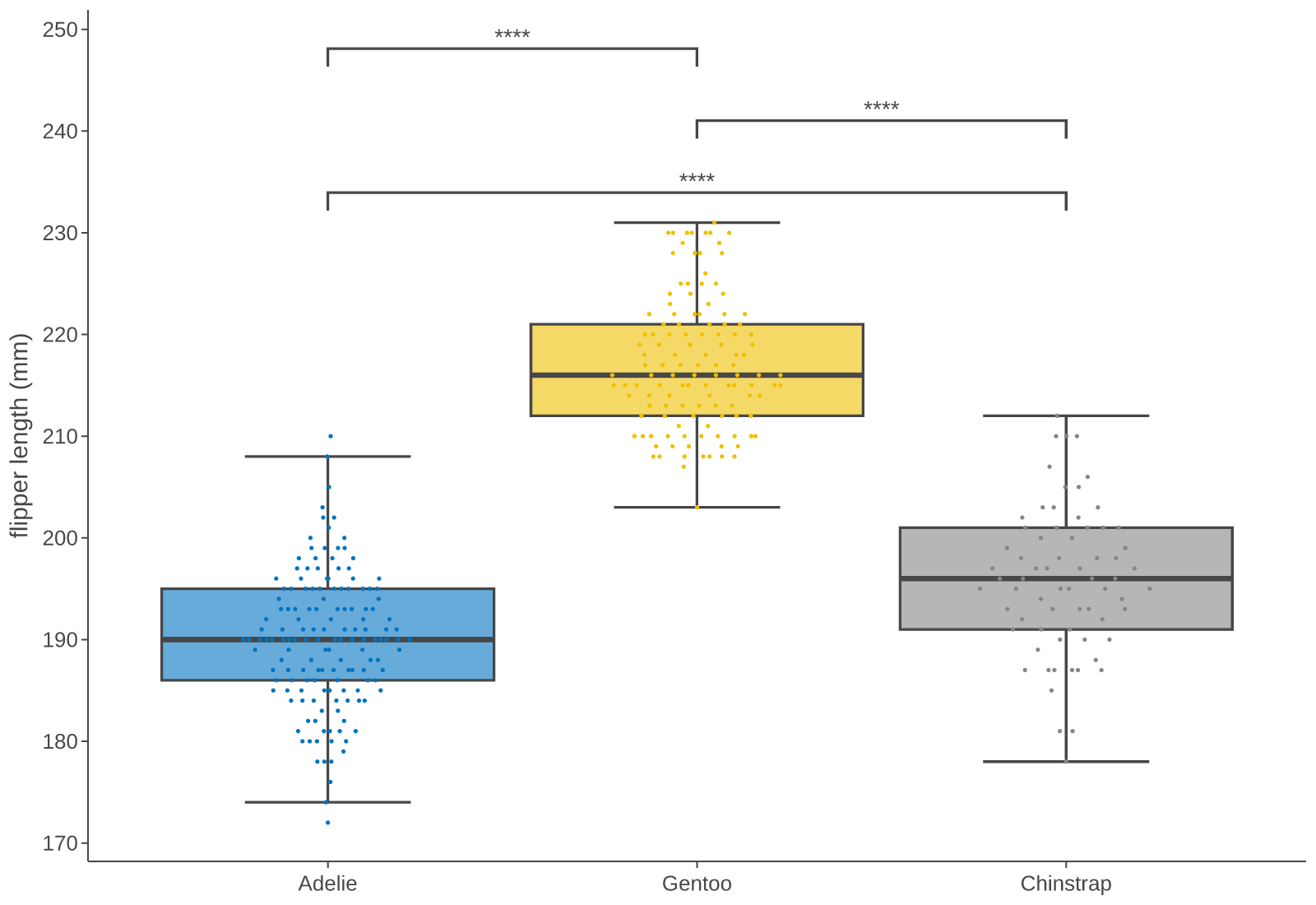
Every plot above is ggrust. More in the gallery.
Highlights
- Fast and lean: at 1M rows a typical plot renders 5x faster than ggplot2 and 90x faster than Lets-Plot, with 4x and 7.5x less memory (benchmarks).
- ggplot2 extensions, built in: beeswarms, significance brackets, cluster marks, side panels, dendrograms, raincloud plots, patchwork layouts and more, under their R names (list).
- The Lets-Plot API: most code ports with an import swap,
lets_plot->ggrust. - Interactive: notebook and HTML output with tooltips, zoom and pan; dense point layers drawn on a canvas.
- Publication output: SVG, PNG, vector PDF and HTML, with your own fonts. Data crosses into Rust once, as Arrow, so Polars and pandas frames work directly.
Installation
pip install ggrust
uv add ggrust
Quickstart
from ggrust import *
from ggrust.data import penguins

plot = (
    ggplot(penguins.drop_nulls(), aes("bill_length_mm", "bill_depth_mm"))
    + geom_smooth(method="lm", color="grey", linetype="dashed", se=False)
    + geom_point(aes(color="species"), size=2.5, alpha=0.7)
    + geom_smooth(aes(color="species", fill="species"), method="lm")
    + stat_cor(aes(color="species"), label_x_npc="right", label_y_npc="bottom")
    + scale_color_npg()
    + scale_fill_npg()
    + labs(
        title="Simpson's paradox in Palmer penguins",
        subtitle="Overall, longer bills look shallower (dashed). Within every species, the opposite.",
        x="bill length (mm)",
        y="bill depth (mm)",
    )
    + theme_classic()
    + ggsize(760, 500)
)

plot.to_png("plot.png")
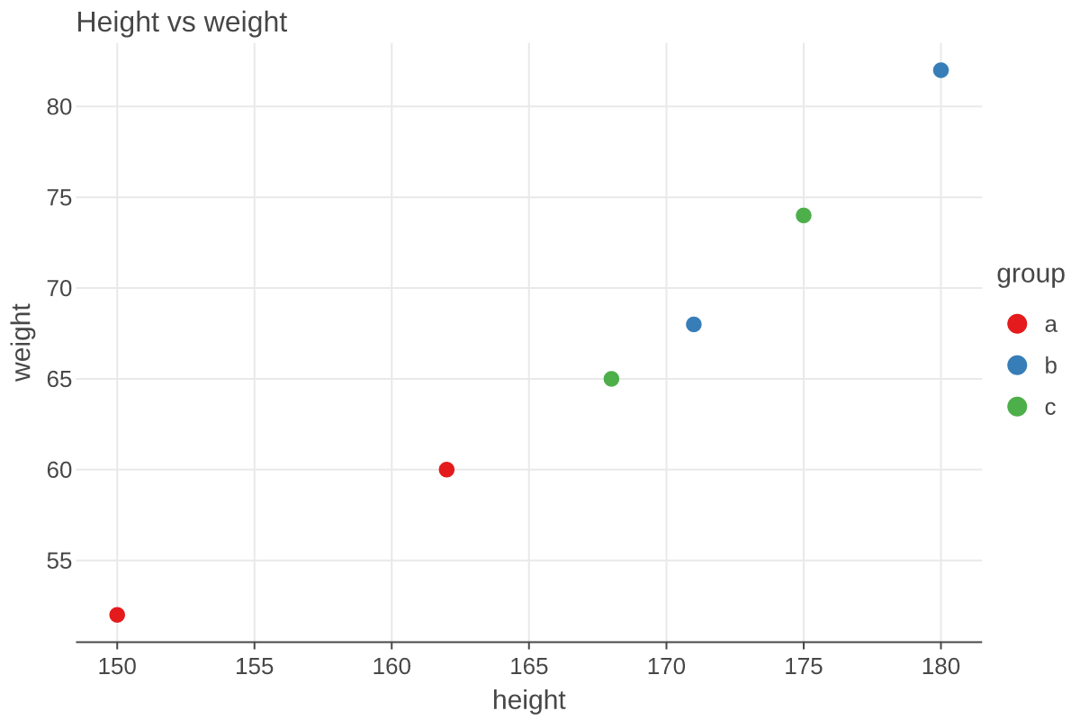
In a notebook the plot shows as interactive HTML (tooltips, zoom and pan with ggtb()).
Showcase
From 3D surfaces to album covers, all drawn with the same + grammar.
3D surface
geom_surface under coord_3d. Neither Lets-Plot nor ggplot2 draws 3D.
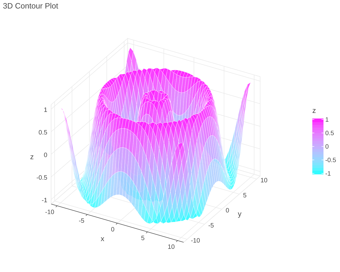
Show code
import numpy as np
from ggrust import *

axis = np.linspace(-10, 10, 40)
x, y = np.meshgrid(axis, axis)
z = np.sin(np.sqrt(x**2 + y**2))
data = {"x": x.ravel(), "y": y.ravel(), "z": z.ravel()}

plot = (
    ggplot(data, aes("x", "y", z="z", fill="z"))
    + geom_surface(alpha=0.8)
    + scale_fill_gradient(low="#00FFFF", high="#FF00FF")
    + coord_3d()
    + ggtitle("3D Contour Plot")
    + ggsize(700, 560)
)
plot
Funky heatmap
The scib single-cell integration benchmark, rebuilt from tiles, points, icons and labels.
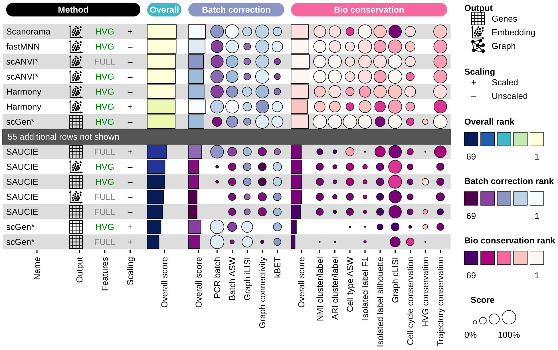
Show code
import polars as pl
from ggrust import *
from ggrust.bistro import funky_heatmap, position_arguments

DATA = "https://raw.githubusercontent.com/datavil/ggrust/main/docs/data/"
runs = pl.read_csv(DATA + "scib_immune.csv")

batch = {
    "PCR_batch": "PCR batch",
    "ASW_label/batch": "Batch ASW",
    "iLISI": "Graph iLISI",
    "graph_conn": "Graph connectivity",
    "kBET": "kBET",
}
bio = {
    "NMI_cluster/label": "NMI cluster/label",
    "ARI_cluster/label": "ARI cluster/label",
    "ASW_label": "Cell type ASW",
    "isolated_label_F1": "Isolated label F1",
    "isolated_label_silhouette": "Isolated label silhouette",
    "cLISI": "Graph cLISI",
    "cell_cycle_conservation": "Cell cycle conservation",
    "hvg_overlap": "HVG conservation",
    "trajectory": "Trajectory conservation",
}
methods = {
    "scanorama": "Scanorama",
    "fastmnn": "fastMNN",
    "scanvi": "scANVI*",
    "harmony": "Harmony",
    "scgen": "scGen*",
    "saucie": "SAUCIE",
}
icons = {"full": "genes", "embed": "embedding", "knn": "graph"}


def rank_color(column: str) -> pl.Expr:
    """Rank 1 (best) -> 1.0 (lightest color), last -> 0.0."""
    rank = pl.col(column).rank("min", descending=True)
    return 1 - (rank - 1) / (rank.max() - 1)


scores = (
    runs.with_columns(
        (pl.col(name) - pl.col(name).min()) / (pl.col(name).max() - pl.col(name).min())
        for name in [*batch, *bio]
    )
    .with_columns(batch=pl.mean_horizontal(*batch), bio=pl.mean_horizontal(*bio))
    .with_columns(overall=0.4 * pl.col("batch") + 0.6 * pl.col("bio"))
    .with_columns(
        rank_color(name).alias(f"{name}_rank") for name in ["overall", "batch", "bio", *batch, *bio]
    )
    .sort("overall", descending=True)
    .with_columns(
        id=pl.int_range(pl.len()).cast(pl.String),
        name=pl.col("method").replace(methods),
        icon=DATA + "scib_icons/" + pl.col("output").replace_strict(icons) + ".png",
        features=pl.col("features").replace({"full_feature": "FULL", "hvg": "HVG"}),
        scaling=pl.col("scaling").replace({"scaled": "+", "unscaled": "\u2013"}),
    )
)
shown = pl.concat([scores.head(7), scores.tail(7)])
separator = pl.DataFrame({"id": ["hidden"]})
table = pl.concat([shown.head(7), separator, shown.tail(7)], how="diagonal_relaxed")


def score(column: str, name: str, geom: str, group: str) -> dict:
    """Describe a score column: its size from ``column``, its color from the rank."""
    width = 2.5 if group == "overall" else 1.5 if geom == "bar" else 1
    return {
        "id": column,
        "id_color": f"{column}_rank",
        "name": name,
        "geom": geom,
        "group": group,
        "palette": group,
        "draw_outline": False,
        "options": {"width": width},
    }


def method(column: str, name: str, geom: str, width: float, **options: object) -> dict:
    """Describe a method column."""
    return {
        "id": column,
        "name": name,
        "geom": geom,
        "group": "method",
        "options": {"width": width, **options},
    }


column_info = [
    method("name", "Name", "text", 4.5, hjust=0),
    method("icon", "Output", "image", 1.5),
    {**method("features", "Features", "text", 2), "palette": "features", "id_color": "features"},
    method("scaling", "Scaling", "text", 1.5),
    score("overall", "Overall score", "bar", "overall"),
    score("batch", "Overall score", "bar", "batch"),
    *[score(column, name, "circle", "batch") for column, name in batch.items()],
    score("bio", "Overall score", "bar", "bio"),
    *[score(column, name, "circle", "bio") for column, name in bio.items()],
]
column_groups = [
    {"header": "Method", "group": "method", "palette": "black"},
    {"header": "Overall", "group": "overall", "palette": "overall"},
    {"header": "Batch correction", "group": "batch", "palette": "batch"},
    {"header": "Bio conservation", "group": "bio", "palette": "bio"},
]


def brewer(codes: str) -> list[str]:
    """Colors from dark (rank 69) to light (rank 1)."""
    return ["#" + code for code in reversed(codes.split())]


palettes = {
    "black": ["black", "black"],
    "features": {"FULL": "#808080", "HVG": "#008000"},
    "overall": brewer("FFFFD9 EDF8B1 C7E9B4 7FCDBB 41B6C4 1D91C0 225EA8 253494 081D58"),
    "batch": brewer("F7FCFD E0ECF4 BFD3E6 9EBCDA 8C96C6 8C6BB1 88419D 810F7C 4D004B"),
    "bio": brewer("FFF7F3 FDE0DD FCC5C0 FA9FB5 F768A1 DD3497 AE017E 7A0177 49006A"),
}
ranks = ["69", "", "", "", "1"]
legends = [
    {
        "title": "Output",
        "geom": "image",
        "labels": [DATA + f"scib_icons/{icon}.png" for icon in icons.values()],
        "values": ["Genes", "Embedding", "Graph"],
    },
    {
        "title": "Scaling",
        "geom": "text",
        "labels": ["+", "\u2013"],
        "values": ["Scaled", "Unscaled"],
    },
    {"title": "Overall rank", "palette": "overall", "geom": "rect", "labels": ranks, "size": 1},
    {
        "title": "Batch correction rank",
        "palette": "batch",
        "geom": "rect",
        "labels": ranks,
        "size": 1,
    },
    {
        "title": "Bio conservation rank",
        "palette": "bio",
        "geom": "rect",
        "labels": ranks,
        "size": 1,
    },
    {"title": "Score", "geom": "circle", "labels": ["0%", "", "", "", "100%"], "color": "white"},
]

heatmap = funky_heatmap(
    table,
    column_info=column_info,
    column_groups=column_groups,
    palettes=palettes,
    legends=legends,
    position_args=position_arguments(
        col_annot_position="bottom",
        col_annot_angle=90,
        col_annot_offset=6,
        col_group_radius=0.5,
        legend_position="right",
        expand_xmax=1,
    ),
    scale_column=False,
    add_abc=False,
)

# The hidden runs: a dark band on the separator row (row 8 is centred at y = -8 x 1.1).
# Its x range is the row background: 0.25 past the first and last column (0.1, 32.3).
hidden = len(scores) - len(shown)
band = pl.DataFrame(
    {
        "xmin": [-0.15],
        "xmax": [32.55],
        "ymin": [-9.35],
        "ymax": [-8.25],
        "x": [0.2],
        "y": [-8.8],
        "label": [f"{hidden} additional rows not shown"],
    }
)
plot = (
    heatmap
    + geom_rect(
        aes(xmin="xmin", xmax="xmax", ymin="ymin", ymax="ymax"),
        data=band,
        fill="#555555",
        color=None,
    )
    + geom_text(aes(x="x", y="y", label="label"), data=band, color="white", hjust=0, size=7.6)
)
plot
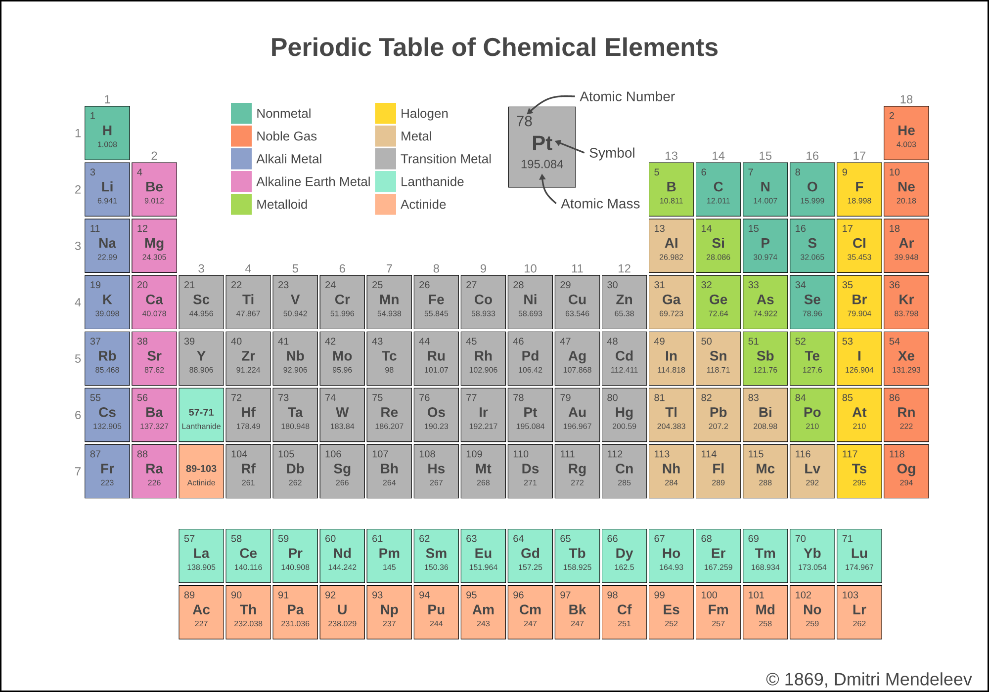
Periodic table
Tiles, text and a hand-placed legend: one ggplot, no images.
Show code
import polars as pl
from ggrust import *

DATA = "https://raw.githubusercontent.com/datavil/ggrust/main/docs/data/"
elements = pl.read_csv(DATA + "elements.csv")

side = 0.95  # tile side, in table cells
key_ratio = 1.5  # the key tile is this much larger
key_x, key_y = 10.25, 1.25

# Lanthanides and actinides go in two rows below the table.
f_block = pl.col("type").is_in(["Lanthanide", "Actinide"])
main = elements.filter(~f_block).with_columns(x=pl.col("group"), y=pl.col("period"))
below = elements.filter(f_block).with_columns(
    x=pl.int_range(pl.len()) % 15 + 3, y=pl.col("period") + 2.5
)
table = pl.concat([main, below], how="vertical_relaxed")
placeholders = pl.DataFrame(
    {"x": [3, 3], "y": [6, 7], "type": ["Lanthanide", "Actinide"], "range": ["57-71", "89-103"]}
)
key = elements.filter(pl.col("atomic_number") == 78).with_columns(x=key_x, y=key_y)
groups = main.group_by("group").agg(y=pl.col("period").min())
periods = pl.DataFrame({"x": [0] * 7, "period": range(1, 8)})
notes = pl.DataFrame(
    {
        "x": [key_x + 0.8, key_x + 1, key_x + 0.4],
        "y": [key_y - 0.9, key_y + 0.1, key_y + 1],
        "label": ["Atomic Number", "Symbol", "Atomic Mass"],
    }
)
hover = (
    layer_tooltips()
    .title("@element\n(@type)")
    .line("Atomic number|@atomic_number")
    .line("Atomic mass|@atomic_mass")
    .line("Electrons|@electron_configuration")
)
head = arrow(angle=30, length=4, type="closed")

plot = (
    ggplot(mapping=aes("x", "y"))
    # The table: atomic number, symbol and mass on each tile.
    + geom_tile(
        aes(fill="type"),
        data=table,
        color="black",
        size=0.25,
        width=side,
        height=side,
        tooltips=hover,
    )
    + geom_text(
        aes(label="atomic_number"),
        data=table,
        nudge_x=-0.37,
        nudge_y=0.37,
        hjust="left",
        vjust="top",
        size=5,
    )
    + geom_text(aes(label="symbol"), data=table, nudge_y=0.05, size=7, fontface="bold")
    + geom_text(aes(label="atomic_mass"), data=table, nudge_y=-0.2, size=4, label_format=".3~f")
    # Where the lanthanides and actinides belong.
    + geom_tile(
        aes(fill="type"),
        data=placeholders,
        color="black",
        size=0.25,
        width=side,
        height=side,
        tooltips="none",
    )
    + geom_text(aes(label="range"), data=placeholders, nudge_y=0.05, size=5, fontface="bold")
    + geom_text(aes(label="type"), data=placeholders, nudge_y=-0.2, size=4)
    # The key: one larger tile with notes and arrows.
    + geom_tile(
        aes(fill="type"),
        data=key,
        color="black",
        size=0.25,
        width=key_ratio * side,
        height=key_ratio * side,
        tooltips="none",
    )
    + geom_text(
        aes(label="atomic_number"),
        data=key,
        nudge_x=-0.37 * key_ratio,
        nudge_y=0.37 * key_ratio,
        hjust="left",
        vjust="top",
        size=5 * key_ratio,
    )
    + geom_text(
        aes(label="symbol"), data=key, nudge_y=0.05 * key_ratio, size=7 * key_ratio, fontface="bold"
    )
    + geom_text(
        aes(label="atomic_mass"),
        data=key,
        nudge_y=-0.2 * key_ratio,
        size=4 * key_ratio,
        label_format=".3~f",
    )
    # Group and period numbers.
    + geom_text(
        aes("group", "y", label="group"),
        data=groups,
        color="gray",
        nudge_y=0.525,
        vjust="bottom",
        size=6,
    )
    + geom_text(
        aes("x", "period", label="period"), data=periods, color="gray", nudge_x=0.375, size=6
    )
    # Notes on the key.
    + geom_text(aes(label="label"), data=notes, hjust=0)
    + geom_curve(
        x=key_x + 0.7,
        y=key_y - 0.9,
        xend=key_x - 0.3,
        yend=key_y - 0.6,
        curvature=0.4,
        ncp=1,
        arrow=head,
    )
    + geom_segment(x=key_x + 0.9, y=key_y + 0.1, xend=key_x + 0.3, yend=key_y - 0.1, arrow=head)
    + geom_curve(
        x=key_x + 0.3,
        y=key_y + 1,
        xend=key_x,
        yend=key_y + 0.5,
        curvature=-0.4,
        ncp=1,
        arrow=head,
    )
    + scale_y_reverse()
    + scale_fill_brewer(name="", type="qual", palette="Set2", guide=guide_legend(ncol=2))
    + coord_fixed(ratio=1.2)
    + labs(title="Periodic Table of Chemical Elements", caption="© 1869, Dmitri Mendeleev")
    + theme_void()
    + theme(
        plot_title=element_text(size=26, face="bold", hjust=0.5, margin=[30, 0, 5, 0]),
        plot_caption=element_text(size=18),
        plot_background=element_rect(color="black", size=3),
        legend_position=[0.36, 0.85],
        legend_background="blank",
    )
    + ggsize(1000, 700)
)
plot
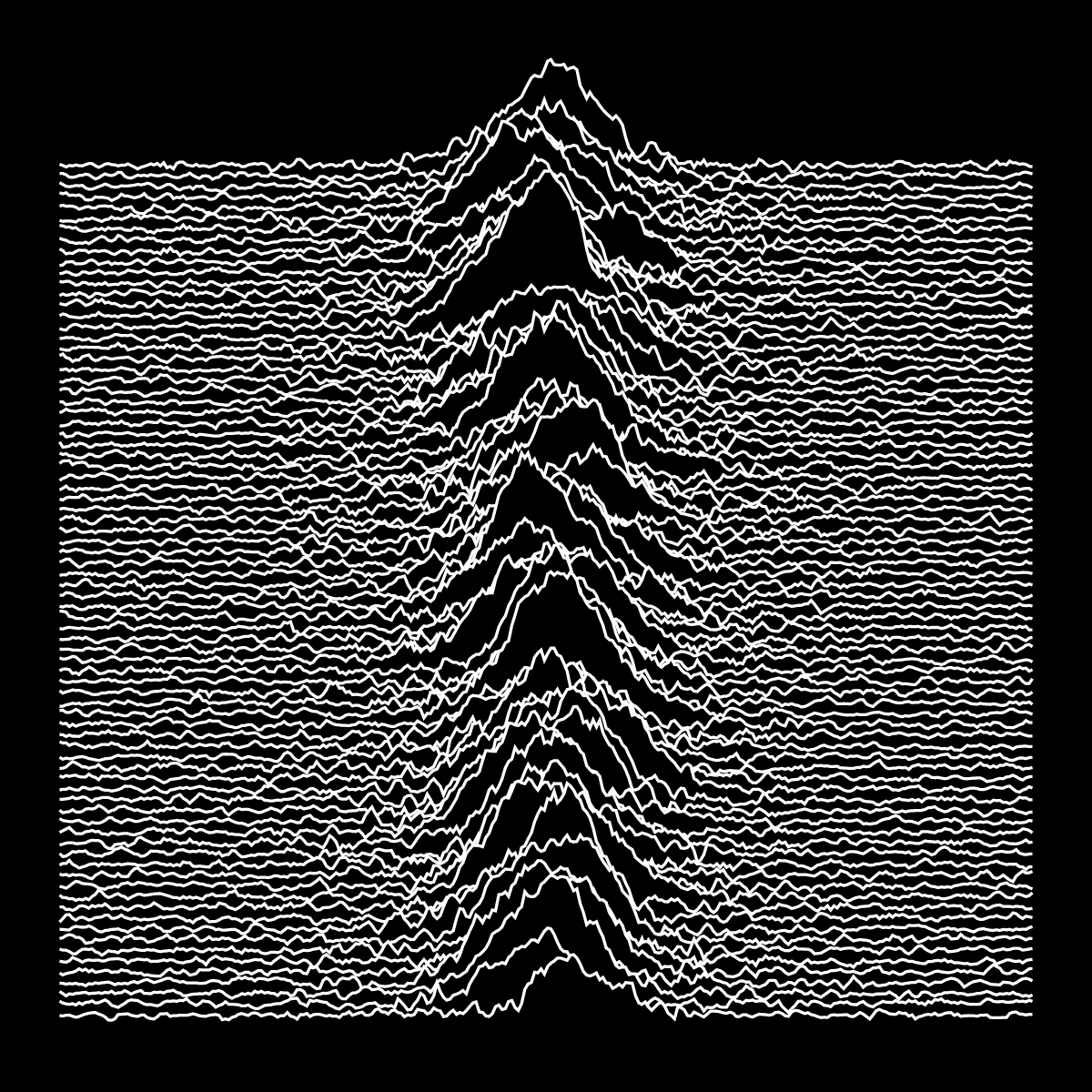
Unknown Pleasures
Simulated pulsar pulses as stacked ridgelines, on a black theme.
Show code
import polars as pl
from ggrust import *

DATA = "https://raw.githubusercontent.com/datavil/ggrust/main/docs/data/"
pulses = pl.read_csv(DATA + "pulsar.csv", has_header=False)
signal = (
    pulses.with_row_index("pulse")
    .unpivot(index="pulse", variable_name="column", value_name="height")
    .with_columns(
        time=pl.col("column").str.strip_prefix("column_").cast(pl.Int64),
        height=pl.col("height") - pl.col("height").min(),
    )
)

plot = (
    ggplot(signal)
    + geom_area_ridges(
        aes("time", "pulse", height="height"),
        stat="identity",
        scale=0.25,
        color="white",
        fill="black",
    )
    + scale_y_reverse()
    + theme_minimal()
    + theme(axis="blank", panel_grid="blank")
    + flavor_high_contrast_dark()
    + ggsize(600, 600)
)
plot
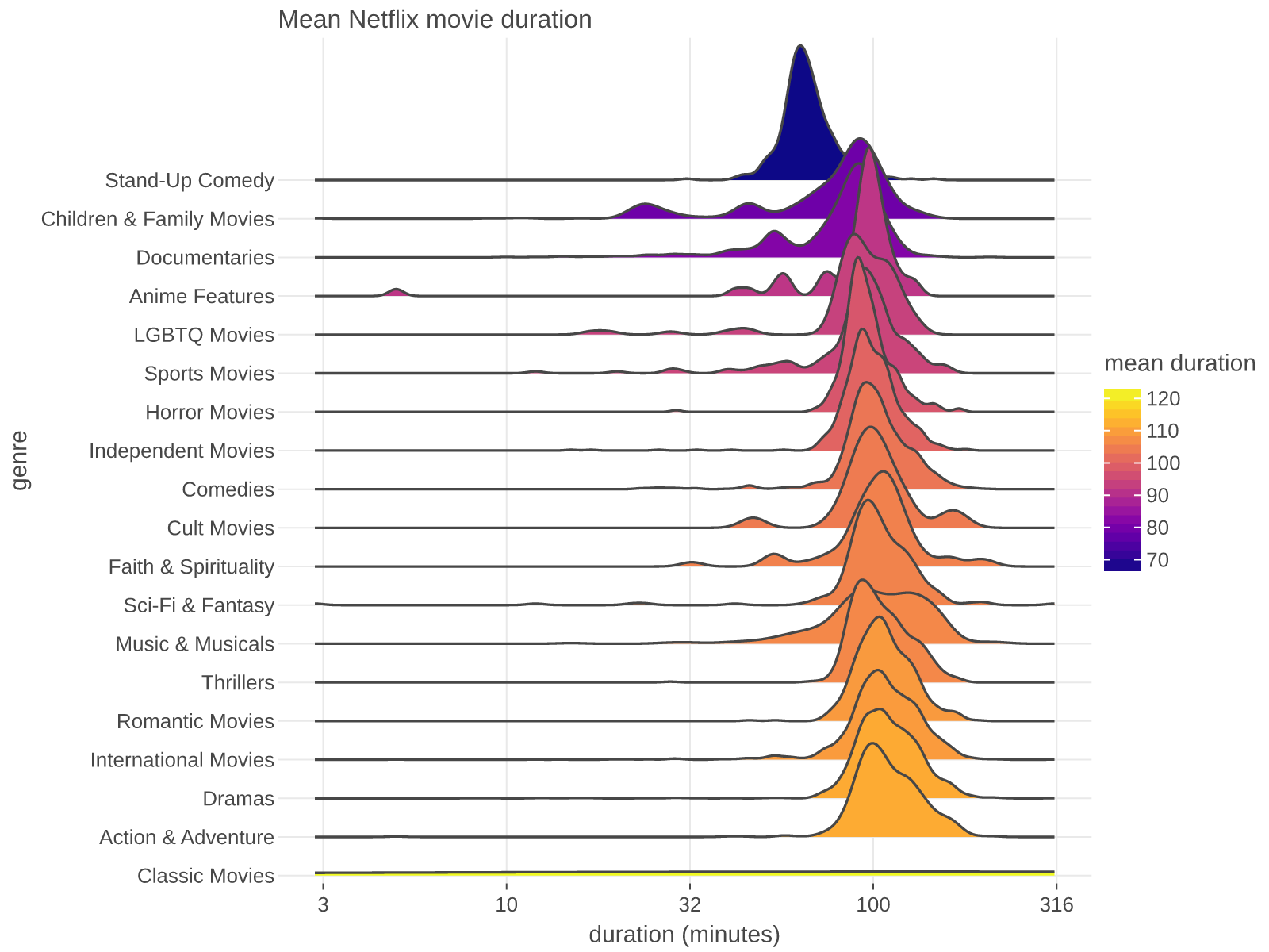
Ridgelines
Netflix movie durations by genre, filled by the genre mean on a log scale.
Show code
import polars as pl
from ggrust import *

DATA = "https://raw.githubusercontent.com/datavil/ggrust/main/docs/data/"
movies = (
    pl.read_csv(DATA + "netflix.csv")
    .filter(pl.col("genres") != "Movies")
    .with_columns(genre=pl.col("genres").str.split(", "))
    .explode("genre", empty_as_null=True)
    .with_columns(mean_minutes=pl.col("minutes").mean().over("genre"))
    .sort("mean_minutes", descending=True)
)

plot = (
    ggplot(movies, aes("minutes", "genre"))
    + geom_area_ridges(
        aes(group="genre", fill="mean_minutes"),
        scale=4,
        tooltips=layer_tooltips().title("@genre").line("duration|@minutes min"),
    )
    + scale_x_log10("duration (minutes)")
    + scale_fill_viridis(name="mean duration", option="plasma")
    + ggtitle("Mean Netflix movie duration")
    + theme(axis_line_x="blank")
    + ggsize(800, 600)
)
plot
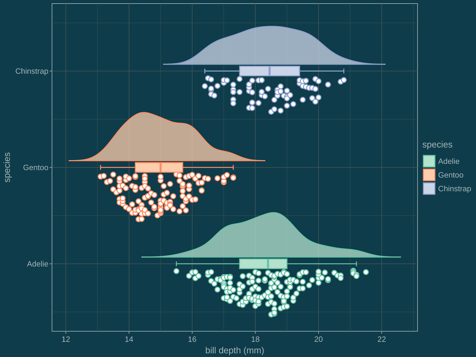
Raincloud
Half violins, sina points and boxplots, on a solarized dark flavor.
Show code
import polars as pl
from ggrust import *

DATA = "https://raw.githubusercontent.com/datavil/ggrust/main/docs/data/"
penguins = pl.read_csv(DATA + "penguins.csv").drop_nulls("bill_depth_mm")

plot = (
    ggplot(penguins, aes("species", "bill_depth_mm", color="species", fill="species"))
    + geom_violin(show_half=1, alpha=0.75, trim=False, position=position_nudge(x=0.07))
    + geom_sina(
        show_half=-1,
        fill="white",
        shape=21,
        seed=42,
        show_legend=False,
        position=position_nudge(x=-0.07),
    )
    + geom_boxplot(width=0.1, outlier_alpha=0, show_legend=False)
    + scale_color_brewer(palette="Set2")
    + scale_fill_brewer(palette="Pastel2")
    + coord_flip()
    + ylab("bill depth (mm)")
    + theme_light()
    + flavor_solarized_dark()
    + ggsize(800, 600)
)
plot
Over 40 more in the gallery, including animations.
ggplot2 extensions, built in
Many popular ggplot2 extension packages from R are built into ggrust, under their R function names. Nothing extra to install; Lets-Plot has none of them.
| Feature | ggrust | From the R package |
|---|---|---|
| Beeswarm and quasirandom points | geom_beeswarm, geom_quasirandom |
ggbeeswarm |
| Journal color palettes | scale_color_npg, _aaas, _nejm, _lancet, _jama, _jco, _d3, _igv |
ggsci |
| Significance tests and labels | stat_compare_means, stat_cor, stat_poly_eq |
ggpubr, ggpmisc |
| Cluster marks | geom_mark_hull, geom_mark_ellipse, geom_mark_rect |
ggforce |
| Highlighting | gghighlight |
gghighlight |
| Point density | geom_pointdensity |
ggpointdensity |
| Side panels | geom_xside*, geom_yside*, ggmarginal |
ggside |
| Several color scales in one plot | new_scale_fill, new_scale_color, new_scale |
ggnewscale |
| Dendrograms | hclust, scale_x_dendro, scale_y_dendro, geom_dendrogram |
legendry, ggh4x, ggdendro |
| Raincloud plots | stat_halfeye, stat_interval, geom_half_violin, geom_half_boxplot, geom_half_point |
ggdist, gghalves |
| Figure layouts and panel tags | gggrid(design=, tag_levels=), inset_element |
patchwork |
| Rasterized layers in vector output | rasterize |
ggrastr, scattermore |
ggrust reimplements their behavior in Rust; the R packages and their authors designed it. Examples and credits are in the extensions guide.
Performance
11 everyday plots (scatter, histogram, boxplot, violin, density, lm smooth, line, 2D bins, facets and more) at 10k, 100k and 1M rows, each saved as SVG and PNG. Same data, every row drawn (Lets-Plot's sampling turned off), same output size, each run in a fresh process. Apple M4 Pro; ggrust main (0.8.0 plus a line-drawing fix), R ggplot2 4.0.1 (svglite, ragg), lets-plot 4.11.0.
| 1M rows | SVG, all 11 plots | PNG, all 11 plots | peak memory per plot |
|---|---|---|---|
| ggrust | 0.91 s | 2.85 s | 138 MB |
| ggplot2 | 9.67 s (10.6x) | 25.0 s (8.8x) | 560 MB |
| Lets-Plot | 71.6 s (78.9x) | > 495 s (> 174x) | 1.0 GB |
- ggrust is faster than both in all 66 cases (11 plots x 3 sizes x 2 formats).
- Lets-Plot did not finish the 1M-row line PNG within 300 s; it counts as 300 s in its total.
Charts, rules and how to reproduce: the benchmarks page. Raw numbers: benchmarks/REPORT-three-way.md.
More examples
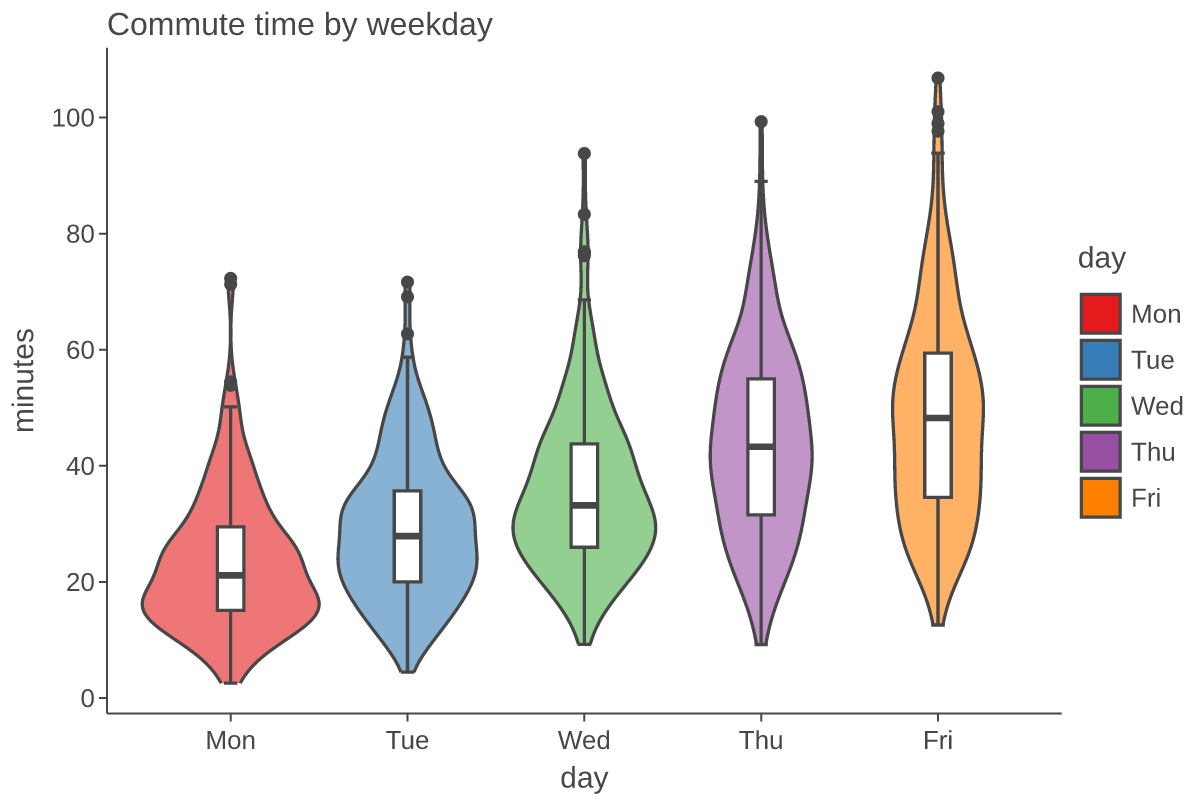
Distributions
Violins with boxplots on top, using the same layering as ggplot.
Show code
import numpy as np

rng = np.random.default_rng(0)
days = ["Mon", "Tue", "Wed", "Thu", "Fri"]
commute = pl.DataFrame(
    {
        "day": np.repeat(days, 200),
        "minutes": np.concatenate([rng.gamma(4 + i, 6, 200) for i in range(5)]),
    }
)

(
    ggplot(commute, aes(x="day", y="minutes", fill="day"))
    + geom_violin(alpha=0.6)
    + geom_boxplot(width=0.15, fill="white")
    + labs(title="Commute time by weekday")
    + theme_classic()
    + ggsize(600, 400)
)
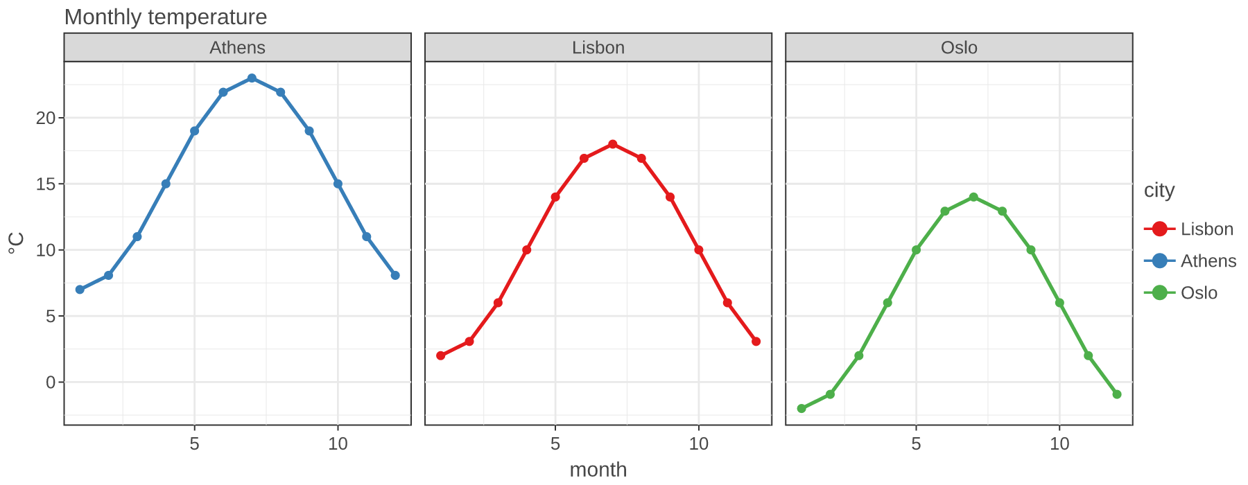
Facets
Split a plot into panels by a column.
Show code
months = np.arange(1, 13)
temperature = pl.DataFrame(
    {
        "month": np.tile(months, 3),
        "temp": np.concatenate(
            [10 + 8 * np.sin((months - 3) / 12 * 2 * np.pi) + offset for offset in (0, 5, -4)]
        ),
        "city": np.repeat(["Lisbon", "Athens", "Oslo"], 12),
    }
)

(
    ggplot(temperature, aes(x="month", y="temp", color="city"))
    + geom_line(size=1.2)
    + geom_point()
    + facet_wrap("city", ncol=3)
    + labs(title="Monthly temperature", y="°C")
    + theme_bw()
    + ggsize(900, 350)
)
What it covers
- Geoms: point, line, path, bar, col, histogram, boxplot, violin, area ridges, tile, raster, rect, text, label, text/label repel, segment, curve, polygon, rug, imshow, brackets and more.
- Stats: count, bin, density, smooth, summary, ecdf, contours, 2D bins, ellipses.
- Scales: continuous, discrete, log, reversed, datetime, hue, manual, gradients, viridis, brewer, secondary axes, axes on any side.
- 3D:
coord_3dwithgeom_surface, beyond both Lets-Plot and ggplot2. - Layout:
facet_wrap,facet_grid,gggridwith collected legends,coord_fixed,coord_flip, themes (theme_classic,theme_bw,theme_minimal,theme_void, ...). - Outputs: SVG, PNG, vector PDF, and interactive HTML through
ggsave, with your own fonts (register_font). Dense scatter layers are drawn on a canvas in HTML.
ggrust is a subset of Lets-Plot, not all of it. Features follow what Cellestial and everyday plotting need. See the migration note for the differences.
Status
Stable from 1.0: names, signatures and error classes are frozen under semantic versioning, while the drawn output can still improve between minor releases (see the stability policy). Animation is provisional. The full Cellestial test suite passes on ggrust. It is a subset of Lets-Plot, so expect gaps; issues are welcome.
Development
uv sync          # create the dev environment
make develop     # build the Rust extension into .venv
make check       # fmt, clippy, ruff, cargo test, pytest
1 maintainer

Metadata
1 maintainer
Release files for ggrust 1.0.0
For a detailed explanation of source distributions (sdists) and built distributions (wheels), please see the package formats documentation.
Source distribution (sdist)
| File | Size | Uploaded | Provenance | Actions |
|---|---|---|---|---|
| ggrust-1.0.0.tar.gz | 3.1 MB | With provenance | Details for ggrust-1.0.0.tar.gz |
Built distributions (wheels)
| File | Actions Reset | |||
|---|---|---|---|---|
| ggrust-1.0.0-cp311-abi3-win_arm64.whl | CPython 3.11 | abi3 | Windows ARM64 | Details for ggrust-1.0.0-cp311-abi3-win_arm64.whl |
| ggrust-1.0.0-cp311-abi3-win_amd64.whl | CPython 3.11 | abi3 | Windows x86-64 | Details for ggrust-1.0.0-cp311-abi3-win_amd64.whl |
| ggrust-1.0.0-cp311-abi3-manylinux_2_28_x86_64.whl | CPython 3.11 | abi3 | Linux glibc 2.28+ x86-64 | Details for ggrust-1.0.0-cp311-abi3-manylinux_2_28_x86_64.whl |
| ggrust-1.0.0-cp311-abi3-manylinux_2_28_aarch64.whl | CPython 3.11 | abi3 | Linux glibc 2.28+ ARM64 | Details for ggrust-1.0.0-cp311-abi3-manylinux_2_28_aarch64.whl |
| ggrust-1.0.0-cp311-abi3-macosx_11_0_arm64.whl | CPython 3.11 | abi3 | macOS 11.0+ ARM64 | Details for ggrust-1.0.0-cp311-abi3-macosx_11_0_arm64.whl |
| ggrust-1.0.0-cp311-abi3-macosx_10_12_x86_64.whl | CPython 3.11 | abi3 | macOS 10.12+ x86-64 | Details for ggrust-1.0.0-cp311-abi3-macosx_10_12_x86_64.whl |
Total release size: 61.4 MB
Release files / ggrust-1.0.0.tar.gz
| Download URL | ggrust-1.0.0.tar.gz |
|---|---|
| Size | 3.1 MB |
| Tags | Source |
|
SHA-256 checksum How to use checksums |
90b9de6fce11c1325d343853edcd040d4992616799a780c621780ad872ee7fee
|
|
BLAKE2b-256 checksum How to use checksums |
e4de04e35216b4d9629953e9f9e77e9b36dc8a28fcf1a6dcecc13f47f20a0d26
|
| Upload date | |
|
Uploaded using Trusted Publishing? What is trusted publishing? |
Yes |
| Uploaded via |
twine/7.0.0 CPython/3.13.16
|
Provenance
Provenance describes where a file came from. On PyPI, provenance is shared via attestations, which provide a verifiable record of the build or publishing details. View details, limitations and caveats.


PyPI Publish Attestation
PyPI verified that this artifact, at this checksum, originated from the publisher listed below.
Signed by GitHub Actions, verified by PyPI on Nov 17, 2026.
Transparency logRelease files / ggrust-1.0.0-cp311-abi3-win_arm64.whl
| Download URL | ggrust-1.0.0-cp311-abi3-win_arm64.whl |
|---|---|
| Size | 9.3 MB |
| Tags | CPython 3.11 Windows ARM64 abi3 |
|
SHA-256 checksum How to use checksums |
49bb40ee832005eb49fe95a652551fd2281772dd7dcf64398aa5bb8765db964e
|
|
BLAKE2b-256 checksum How to use checksums |
8324cb8267f8ca4e27783e033a15ed9d7e94359682ac171197e620ab7d634797
|
| Upload date | |
|
Uploaded using Trusted Publishing? What is trusted publishing? |
Yes |
| Uploaded via |
twine/7.0.0 CPython/3.13.16
|
Provenance
Provenance describes where a file came from. On PyPI, provenance is shared via attestations, which provide a verifiable record of the build or publishing details. View details, limitations and caveats.
PyPI Publish Attestation
PyPI verified that this artifact, at this checksum, originated from the publisher listed below.
Signed by GitHub Actions, verified by PyPI on Nov 17, 2026.
Transparency logRelease files / ggrust-1.0.0-cp311-abi3-win_amd64.whl
| Download URL | ggrust-1.0.0-cp311-abi3-win_amd64.whl |
|---|---|
| Size | 10.2 MB |
| Tags | CPython 3.11 Windows x86-64 abi3 |
|
SHA-256 checksum How to use checksums |
e6292683b4b1f5a87fa408331c71c6d38be3021b0d357c848d3dab373adef7c3
|
|
BLAKE2b-256 checksum How to use checksums |
c77aad8bff2bcb1e2d0cf0656630c9d021db7f2491ce357fe720099687c66c54
|
| Upload date | |
|
Uploaded using Trusted Publishing? What is trusted publishing? |
Yes |
| Uploaded via |
twine/7.0.0 CPython/3.13.16
|
Provenance
Provenance describes where a file came from. On PyPI, provenance is shared via attestations, which provide a verifiable record of the build or publishing details. View details, limitations and caveats.
PyPI Publish Attestation
PyPI verified that this artifact, at this checksum, originated from the publisher listed below.
Signed by GitHub Actions, verified by PyPI on Nov 17, 2026.
Transparency logRelease files / ggrust-1.0.0-cp311-abi3-manylinux_2_28_x86_64.whl
| Download URL | ggrust-1.0.0-cp311-abi3-manylinux_2_28_x86_64.whl |
|---|---|
| Size | 10.1 MB |
| Tags | CPython 3.11 Linux glibc 2.28+ x86-64 abi3 |
|
SHA-256 checksum How to use checksums |
31bc2945851c821e069c7bb05e64562aa6723e21ddb8f8f2cd3043d518dec5d7
|
|
BLAKE2b-256 checksum How to use checksums |
af3164db4c179e384c0a5d3e92f977566a7e54ce29a36e6324f01878086f3d3e
|
| Upload date | |
|
Uploaded using Trusted Publishing? What is trusted publishing? |
Yes |
| Uploaded via |
twine/7.0.0 CPython/3.13.16
|
Provenance
Provenance describes where a file came from. On PyPI, provenance is shared via attestations, which provide a verifiable record of the build or publishing details. View details, limitations and caveats.
PyPI Publish Attestation
PyPI verified that this artifact, at this checksum, originated from the publisher listed below.
Signed by GitHub Actions, verified by PyPI on Nov 17, 2026.
Transparency logRelease files / ggrust-1.0.0-cp311-abi3-manylinux_2_28_aarch64.whl
| Download URL | ggrust-1.0.0-cp311-abi3-manylinux_2_28_aarch64.whl |
|---|---|
| Size | 9.7 MB |
| Tags | CPython 3.11 Linux glibc 2.28+ ARM64 abi3 |
|
SHA-256 checksum How to use checksums |
385cc5de729298abd1ceb021c996e7759a3eae7ec5b5374d03c052b0553e58ab
|
|
BLAKE2b-256 checksum How to use checksums |
cc9dcfba0c1b49901f82e24379dc243d708e948be8936fcd45448be8c0a8886d
|
| Upload date | |
|
Uploaded using Trusted Publishing? What is trusted publishing? |
Yes |
| Uploaded via |
twine/7.0.0 CPython/3.13.16
|
Provenance
Provenance describes where a file came from. On PyPI, provenance is shared via attestations, which provide a verifiable record of the build or publishing details. View details, limitations and caveats.
PyPI Publish Attestation
PyPI verified that this artifact, at this checksum, originated from the publisher listed below.
Signed by GitHub Actions, verified by PyPI on Nov 17, 2026.
Transparency logRelease files / ggrust-1.0.0-cp311-abi3-macosx_11_0_arm64.whl
| Download URL | ggrust-1.0.0-cp311-abi3-macosx_11_0_arm64.whl |
|---|---|
| Size | 9.3 MB |
| Tags | CPython 3.11 abi3 macOS 11.0+ ARM64 |
|
SHA-256 checksum How to use checksums |
049306d2eca0c07aa51664a85678e096b841a7c213181f5d621e9bbf2e3862f6
|
|
BLAKE2b-256 checksum How to use checksums |
26532098059644190bee3666dd10c780913b09d2dd8276035da3922a7972bf41
|
| Upload date | |
|
Uploaded using Trusted Publishing? What is trusted publishing? |
Yes |
| Uploaded via |
twine/7.0.0 CPython/3.13.16
|
Provenance
Provenance describes where a file came from. On PyPI, provenance is shared via attestations, which provide a verifiable record of the build or publishing details. View details, limitations and caveats.
PyPI Publish Attestation
PyPI verified that this artifact, at this checksum, originated from the publisher listed below.
Signed by GitHub Actions, verified by PyPI on Nov 17, 2026.
Transparency logRelease files / ggrust-1.0.0-cp311-abi3-macosx_10_12_x86_64.whl
| Download URL | ggrust-1.0.0-cp311-abi3-macosx_10_12_x86_64.whl |
|---|---|
| Size | 9.8 MB |
| Tags | CPython 3.11 abi3 macOS 10.12+ x86-64 |
|
SHA-256 checksum How to use checksums |
663315ee0e104904353d361af6a8cfd0444b6ac6781b29047b99b68d875afb81
|
|
BLAKE2b-256 checksum How to use checksums |
0411b6a8aa969d2cf1f3582848157602403c5cfc342017a9feca57a34836962e
|
| Upload date | |
|
Uploaded using Trusted Publishing? What is trusted publishing? |
Yes |
| Uploaded via |
twine/7.0.0 CPython/3.13.16
|
Provenance
Provenance describes where a file came from. On PyPI, provenance is shared via attestations, which provide a verifiable record of the build or publishing details. View details, limitations and caveats.
PyPI Publish Attestation
PyPI verified that this artifact, at this checksum, originated from the publisher listed below.
Signed by GitHub Actions, verified by PyPI on Nov 17, 2026.
Transparency logSecurity for ggrust 1.0.0
Provenance
Provenance describes where a file came from. On PyPI, provenance is shared via attestations, which provide a verifiable record of the build or publishing details. View details, limitations and caveats.
Full provenance
All 7 files in this release have been uploaded with provenance metadata.
Attestation for ggrust-1.0.0.tar.gz
PyPI Publish Attestation
PyPI verified that this artifact, at this checksum, originated from the publisher listed below.
Signed by GitHub Actions, verified by PyPI on Nov 17, 2026.
Transparency logA note on package security
PyPI is a repository for distributing packages, not a service for auditing them. While third-party security researchers and our staff do their best to detect and remove malicious packages, PyPI cannot guarantee the quality, security or suitability of any given package.
To learn more about protecting yourself from malicious actors, visit our package security documentation.














