gnuplot-manager 0.1.6

A manager to symplify the use of gnuplot inside python

Contents

• Introduction

• Package structure

• Importing the package

  • How to import

  • Checking gnuplot installation at the module import

• Creating a new plot window

  • The new_plot() function

  • Errors during window creation

  • Persistence

  • Gnuplot output management

  • Purging data files

  • Other plot window properties

  • Default window properties

• Plotting from data

  • Plotting 2D curves from data

  • Plotting 1D data

  • Plotting histograms

  • Plotting boxplots

  • Plotting 3D data

  • Adding more curves to a plot

  • Plotting several curves at the same time

  • Data files

  • Plotting volatile data

• Plotting mathematical functions

  • Plotting a mathematical expression

  • Adding a mathematical expression

  • Plotting several mathematical expressions

• Checking window properties

  • Printing information on a plot window

  • Printing information on all plot windows

• Closing plot windows

  • Closing a single plot window

  • Effects of removing plot window names

  • Deleting the output files

  • Closing all the open windows at once

• Performing other actions

  • Changing the window properties

  • Refreshing windows

  • Resetting windows

  • Printing a label on the plot window

  • Exporting a plot window to a file

  • Exporting all the plot windows

  • Sending arbitrary commands to gnuplot

• List of available functions

  • Create, modify, and close plot windows

  • Plot data

  • Plot mathematical functions

  • Print plots to files

  • Reset, clear and refresh plots

  • Utility functions

• The _PlotWindow class

Introduction

This package allows to plot data or mathematical expressions inside python, using the gnuplot program, in the form of 2D or 3D plots.

Multiple plot windows can be opened, and a separate gnuplot process is started for each of them. The data to be plotted can be transferred to gnuplot by writing them on files, or can be sent to gnuplot inline. Mathematical expressions are sent directly to gnuplot as strings. All the package functionalities can be accessed by calling functions, the list of which is reported in the List of available functions section at the end of this document.

The package has been designed starting from my own needs, so only a very limited number of the many gnuplot functionalities have been implemented, but more may be added in the future:

• plotting 2D or 3D graphs from data

• plotting mathematical expressions in 2D or 3D

The most commonly used plot settings, such as applying logarithmic scales or setting scale limits, can be applied by passing arguments to the functions, without knowing the specific gnuplot commands. However, it is also possible to pass arbitrary commands to gnuplot, as described in the section Sending arbitrary commands to gnuplot.

The examples given in this document can be executed by copying the expressions after ‘>>>’ and pasting them in the python console command line. Note that, although they have been tested, errors are still possible.

Note

If the package has been correctly installed, a small demo script can be run from the system terminal by typing:

$ python -m gnuplot_manager.demo

or inside the python console by typing:

>>> from gnuplot_manager.demo import main
>>> main()

The demo will run without the need of any input.

This package is released under a GPL licence, in the hope it can be useful to someone else. Feeback, bug reports, and suggestions are welcome.

Package structure

This package contains the following modules:

global_variables.py

contains the global variables, mainly used to define default values of some parameters;

errors.py

contains error messages returned by the package functions;

classes.py

contains the _PlotWindow class, used to create a structure containing the gnuplot process (instance of subprocess.Popen) and some information on the plot;

functions.py

contains all the functions used to create plot windows and plot data or mathematical expressions on them;

funcutils.py

contains some utility functions which are not intended to be called directly by the user;

demo.py

a small demo script;

test.py

a script to test most of the package functions.

Importing the package

How to import

To import gnuplot_manager you can use the import directive as usual:

>>> import gnuplot_manager

or

>>> import gnuplot_manager as gm

or also

>>> from gnuplot_manager import *

Note

If you are using this module together with matplotlib, e.g. during an ipython session opened with the –pylab option, it is recommended that you import gnuplot_manager in its own namespace (using one of the two first methods listed above) to prevent any conflict with matplotlib functions and variable names. Efforts have been made to avoid the use of names that could override matplotlib ones (such as plot()), but something may have been forgotten, and future versions of matplolib could use names that conflict with this package. If you import the package in its own namespace, you are sure to avoid any conflict.

Note

In the following, all the examples are written presuming that the package and numpy have been imported in their own namespaces as follows:

>>> import numpy
>>> import gnuplot_manager as gm

numpy is used in the examples to generate some data to be plotted, but the gnuplot_manager package does not rely on it, and the plot functions can handle lists, tuples, or other types of data.

Checking gnuplot installation at the module import

When the module is imported, it checks the availability of the gnuplot program and sets the global variable gnuplot_installed accordingly. This is achieved by means of a call to the program which, that should be installed in nearly all linux distributions. However, if it is not installed on your system, the gnuplot_installed variable is set to None:

gnuplot_installed=True

gnuplot is installed

gnuplot_installed=False

gnuplot is not installed

gnuplot_installed=None

which was not found, so the installation of gnuplot was not checked

Example:

>>> print(gm.gnuplot_installed)
True

Creating a new plot window

The new_plot() function

To open a new plot window, use the new_plot() function

>>> myplot2d = gm.new_plot(plot_type='2D', title='My 2D Plot')

The function returns an instance of the _PlotWindow class. Note that the plot window does not appear on the screen until you plot something on it.

You can specify 2 types of plot: ‘2D’ and ‘3D’, with ‘2D’ as default. If you give a title to the window, passing the title argument to the new_plot() function, it will be shown on the window, when something will be plotted on it. All the arguments are optional: if the function is called without passing any argument, it returns a ‘2D’ plot without a title.

Note

In the following, the options of the new_plot() function are explained: if you want to learn immediately how to plot something, jump to the Plotting from data or Plotting mathematical functions sections.

Errors during window creation

If invalid or inconsisted arguments are given to the new_plot() function, a plot window is created using default values, and a tuple with a number and an error message is stored in the error attribute of the _PlotWindow instance. Examples:

>>> myplot = gm.new_plot(plot_type='4D')
>>> print(myplot.error)
(14, 'unknown plot type "4D", using default "2D"')

Persistence

If you give the persistence=True argument when opening a new plot, the window will remain visible after the gnuplot process has been terminated, as described in the Closing plot windows section. However, some operations, such as zooming and rescaling, may not be possible after the gnuplot process has been shut down.

>>> myplot = gm.new_plot(title='Persistent plot', persistence=True)

The default behavior is stored in the PERSISTENCE global variable:

>>> print(gm.PERSISTENCE)
False

Gnuplot output management

When you open a new plot window, you can specify how you like to treat the output of the associated gnuplot process, passing the redirect_output argument to the new_plot() function:

redirect_output = False

gnuplot output and errors are sent to /dev/stdout and /dev/stderr respectively, as it would happen when calling the program from the terminal. This can be useful when using gnuplot from the console, to get the output immediately;

redirect_output = True

the output is saved to files, which are stored in the directories gnuplot.out/output/ and gnuplot.out/errors/;

redirect_output = None

the output is suppressed, sending it to /dev/null.

You can specify a different behavior for each window you open:

>>> myplot1 = gm.new_plot(title='Output suppressed', redirect_output=None)
>>> myplot2 = gm.new_plot(title='Output saved on files', redirect_output=True)
>>> myplot3 = gm.new_plot(title='Output shown on console', redirect_output=False)

The default behavior is stored in the REDIRECT_OUT global variable:

>>> print(gm.REDIRECT_OUT)
False

Note

By default, gnuplot directs to /dev/stderr the output of some of its commands, such as print, not only errors. As an example, if you press the h key when the mouse pointer is inside a gnuplot window, gnuplot prints a list of the available commands. However, if the redirect_output=True has been specified, the menu appears on the file on which the /dev/stderr (and not /dev/stdout, as one would expect) has been redirected. This depends on the gnuplot behavior and is not due to an erroneous redirection of the devices to the files.

Purging data files

By default, the old datafiles are removed each time new data or functions are plotted on the plot window, unless the replot=True option is given [1]. If you want to change this behavior, preserving the data files, you can pass the purge=False argument to the new_plot() function.

[1]

a description of the replot argument is given in the Adding more curves to a plot section.

Other plot window properties

While opening the plot window, you can specify several other properties, such as: type of terminal, window dimensions, position on the screen, axis limits, labels, and so on.

Read the docstring of the new_plot() function for a list of all the available options (press q to exit from the help page):

>>> help(gm.new_plot)

Default window properties

The default values used by the new_plot() function for terminal type, window dimensions and window position on the screen are not the default ones used by newplot. They are stored in the following global variables:

• DEFAULT_TERM

• DEFAULT_WIDTH

• DEFAULT_HEIGHT

• DEFAULT_XPOS

• DEFAULT_YPOS

the first one is a string (e.g. ‘x11’), while the other ones are numbers expressing the window position and size in pixels.

If you want to open a plot window using gnuplot defaults, you can pass the gnuplot_default argument:

>>> myplot = gm.new_plot(gnuplot_default=True, title='Using gnuplot defaults')

Note

If you have tried some of the examples described up to now, you have opened several _PlotWindow instances, none of which has opened a window on the screen, since there is nothing plotted yet. You can close all the open plot windows, terminating the associated gnuplot terminals, using the plot_close_all() function, described in the Closing plot windows section:

>>> gm.plot_close_all()
(0, 'Ok')

Plotting from data

Plotting 2D curves from data

Before plotting 2D data, a 2D plot window must be opened first, as was described in the Creating a new plot window section:

>>> myplot2d = gm.new_plot(plot_type='2D', title='My 2D Plot')

To plot 2D data, use the plot2d() function, passing the _PlotWindow instance as first argument. The second and third arguments must be unidimensional data structures, such as numpy arrays, lists or tuples [2], having equal sizes, containing the x-values and y-values of the points to plot. As an example, if the second and third argument are two arrays x and y:

• the first point to plot has coordinates (x[0], y[0])

• the second point has coordinates (x[1], y[1])

• and so on…

[2]

even single numbers, if you want to plot a single point.

The third argument (optional) is a string to be used as label in the plot legend. Example:

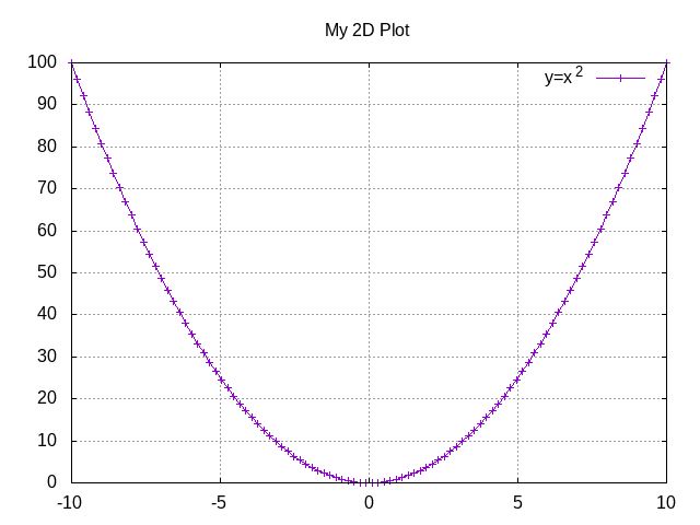
>>> x = numpy.linspace(0,100,1001)
>>> y = x * x
>>> gm.plot2d(myplot2d, x, y, label='y=x^2')
(0, 'Ok')

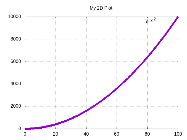
a gnuplot window should appear on the screen, and a parabola should be plotted on it. The plot2d() function returns a tuple containing a number and a string: if there are no errors, the number is zero and the string is ‘Ok’, otherwise a number greater than zero and a string describing the error are returned.

The list of all the error messages is contained in the error.py module:

>>> help(gm.errors)

Plotting 1D data

It is also possible to give to gnuplot a single set of data, usually if you want to give y-values and let gnuplot automatically create the x-values, by means of the plot_1d() function. The function works for 2D plot windows only. Example:

>>> y = numpy.linspace(0,100,101)
>>> gm.plot1d(myplot2d, y, label='1D data')
(0,'Ok')

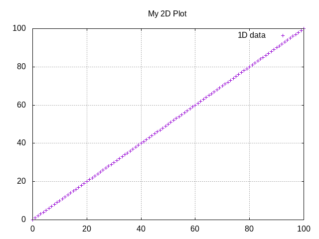
In the previous example gnuplot has used the ordinal numbers 1-100 as x-values for the points of the plot.

Plotting histograms

The plot2d() function can be used to plot histograms also. If the plot was opened passing the argument style=’histeps’, the data are plotted as an histogram, where each x-value is interpreted as the center value of the bin, and each y-value as the associated frequency. Example:

>>> myhistogram = gm.new_plot(style='histeps', title='My Histogram')
>>> bins = [1, 2, 3, 4, 5, 6, 7, 8, 9]
>>> freq = [1, 1, 4, 7, 8, 6, 3, 1, 0]
>>> gm.plot2d(myhistogram, bins, freq, label='My frequency data')
(0,'Ok')

an histogram should be plotted. Note that, in this case, we have put the x and y values in lists, instead of numpy arrays, but we could have put them in tuples also, obtaining the same effect.

You can set the ‘histeps’ style on an already opened 2D plot window also, using the plot_set() function described in the Changing the window properties section.

Plotting boxplots

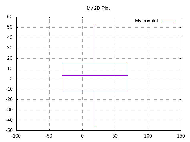
The function plot_box() allows to plot a boxplot from a set of data. Example:

>>> data = numpy.random.normal(3,20,50)
>>> gm.plot_box(myplot2d, data, width=100, label='My boxplot')
(0,'Ok')

Plotting 3D data

To plot 3D data, the plot window must be opened with the option plot_type = ‘3D’, as described in the Creating a new plot window section:

>>> myplot3d = gm.new_plot(plot_type='3D', title='3D Plot')

then, the plot3d() function can be used to plot data on the window, passing the _PlotWindow instance as first argument, and the x, y and z values of the points to plot as the following arguments.

The x, y and z values to be plotted must be stored in unidimensional data structures of equal sizes, and contain the x, y, and z coordinates of each point to plot. As an example, if you pass the three arrays x, y and z:

• the first point to plot has coordinates (x[0], y[0], z[0])

• the second point has coordinates (x[1], y[1], z[1])

• and so on…

Example of 3D curve plot:

>>> x = numpy.linspace(0,100,1001)
>>> y = numpy.linspace(0,200,1001)
>>> z = x * y
>>> gm.plot3d(myplot3d, x, y, z, label='3D curve')
(0, 'Ok')

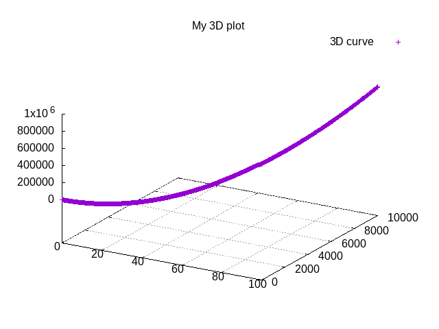
a 3D plot with a curve is plotted. If you click with the mouse on the window and move the pointer, you can rotate the axes, changing the point of view (this is made by gnuplot, not by this package).

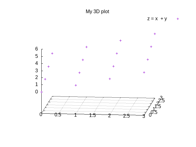
In the previous example, a curve in 3D is plotted, not a surface, since only a single y value is given for each x value. To plot a surface, you must provide a set of y values for each x value, to form a grid of values on the x-y plane. Example of the points needed to plot a z=x+y surface on a grid of 4 x 4 points:

(x=0, y=0, z=0) (x=0, y=1, z=1) (x=0, y=2, z=2) (x=0, y=3, z=3)
(x=1, y=0, z=1) (x=1, y=1, z=2) (x=1, y=2, z=3) (x=1, y=3, z=4)
(x=2, y=0, z=2) (x=2, y=1, z=3) (x=2, y=2, z=4) (x=2, y=3, z=5)
(x=3, y=0, z=3) (x=3, y=1, z=4) (x=3, y=2, z=5) (x=3, y=3, z=6)

So the data to give to the plot3d() functions are:

>>> x = numpy.array([0, 0, 0, 0, 0, 1, 1, 1, 1, 1, 2, 2, 2, 2, 2, 3, 3, 3, 3, 3])
>>> y = numpy.array([0, 1, 2, 3, 0, 1, 2, 3, 0, 1, 2, 3, 0, 1, 2, 3, 0, 1, 2, 3])
>>> z = x + y
>>> gm.plot3d(myplot3d, x, y, z, label='z = x  + y')
(0, 'Ok')

A grid of crosses should be plotted, which are points of the z = x + y surface:

Adding more curves to a plot

To add new data on the same plot, you must pass the replot=True argument:

>>> x1 = numpy.linspace(0,100,1001)
>>> y1 = x1 * x1
>>> gm.plot2d(myplot2d, x1, y1, label='My first 2D data')
(0, 'Ok')
>>> x2 = numpy.linspace(0,100,2001)
>>> y2 = x2 * x2 * x2 / 100
>>> gm.plot2d(myplot2d, x2, y2, label='My second 2D data', replot=True)
(0, 'Ok')

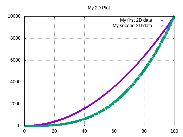
However, if you want to plot multiple curves on the same plot, it is more efficient to use the plot_curves() function described in the next section.

Plotting several curves at the same time

The function plot_curves() allows to plot several curves at one time, which is faster than plotting them one at a time using the replot option, since gnuplot is called only once. Moreover, it lets you add a string with arbitrary options to give to gnuplot.

Data to be plotted must be recorded in a list, each element of which is itself a list, made of 4 elements for 2D plots, or 5 elements for 3D ones.

For 2D plots, each list element has the form [x, y, label, options], while for 3D plots it has the form [x, y, z, label, options], where:

• x is the array of x coordinates of the points to plot: for 2d plot windows it can also be set to None, in which case the x-values for that curve are automatically created by gnuplot;

• y is the array of y coordinates of the points to plot;

• z is the array of z coordinates of the points to plot (only for 3D plots);

• label is a string with the label to show in the plot legend, or None if you do not want a label to be set

• options is a string with additional options you want to give to gnuplot, [3] or None if you do not want to give them

[3]

note that no check is made that the string contains valid gnuplot options.

Examples:

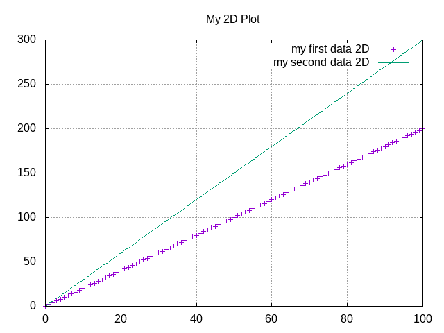
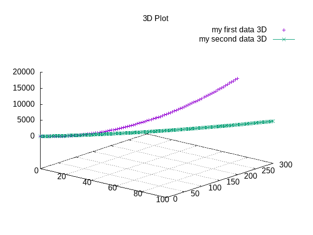
>>> x1 = numpy.linspace(0, 100, 101)
>>> y1 = 2 * x1
>>> z1 = x1 * y1
>>> x2 = numpy.linspace(0, 100, 201)
>>> y2 = 3 * x2
>>> z2 = x2 * y2 / 10
>>> list2d = [ [x1, y1, 'my first data 2D', None], [x2, y2, 'my second data 2D', 'with lines'] ]
>>> list3d = [ [x1, y1, z1, 'my first data 3D', None], [x2, y2, z2, 'my second data 3D', 'with linespoints'] ]

The first argument passed to plot_curves() must be the plot on which you want to operate, while the second is the list:

>>> gm.plot_curves(myplot2d, list2d)
(0, 'Ok')

>>> gm.plot_curves(myplot3d, list3d)
(0, 'Ok')

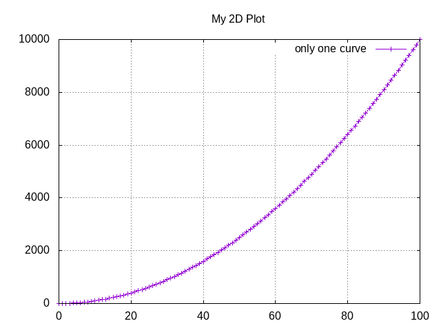
You can also use the function plot_curves() to plot a single curve, which allows to give additional options to gnuplot, but then the list must have a single element, which is itself a list of 4 or 5 elements, so do not forget to put double square brackets:

>>> x1 = numpy.linspace(0,100,101)
>>> y1 = x1 * x1
>>> gm.plot_curves(myplot2d, [ [ x1, y1, 'only one curve', 'with linespoints'] ])
(0, 'Ok')

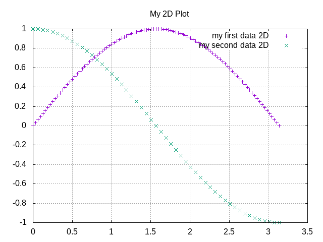
You can specify the replot=True option in the plot_curves() function also, if you want to add the new curves to the previously plotted ones. Example:

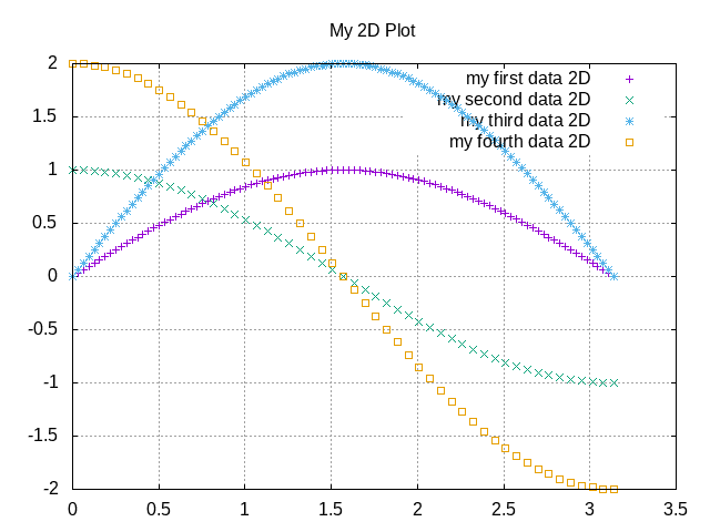
>>> x1 = numpy.linspace(0,3.14, 101)
>>> y1 = numpy.sin(x1)
>>> x2 = numpy.linspace(0,3.14, 51)
>>> y2 = numpy.cos(x2)
>>> list2da = [ [x1, y1, 'my first data 2D', None], [x2, y2, 'my second data 2D', None] ]
>>> list2db = [ [x1, 2*y1, 'my third data 2D', None], [x2, 2*y2, 'my fourth data 2D', None] ]
>>> gm.plot_curves(myplot2d, list2da)
(0, 'Ok')

>>> gm.plot_curves(myplot2d, list2db, replot=True)
(0, 'Ok')

Data files

The data to be plotted are written on files, which are saved in the gnuplot.out/data/ directory, which is created in the current working directory. The name of a data file has the following form:

gnuplot_data_w<n>(<window-title>)_<type>_c<m>(<curve-label>).csv

• <n> is the window number

• <window-title> is the string given to the new_plot() function as window title

• <type> is ‘1D’, ‘2D’ or ‘3D’, where ‘1D’ means that the x-values have been omitted

• <m> is the curve number

• <curve-label> is the string given to the plot function as label

If the window title and/or the curve label have not been given, the filename will miss one or both the parts beween parentheses.

Note that, when composing filenames, characters listed in the INVALID_CHARS global variable are removed from the window titles and curve labels, and substituted with the char stored in the SUBSTITUTE_CHAR variable (which is “_”, unless you change it).

Plotting volatile data

It is also possibile to pass data to gnuplot without writing them to disk. This can be achieved by passing the volatile=True argument to any of the plot functions described in this section. In this case a data file is not created, instead the data are passed to gnuplot as a string, together with the plotting commands, using the special filename ‘-’.

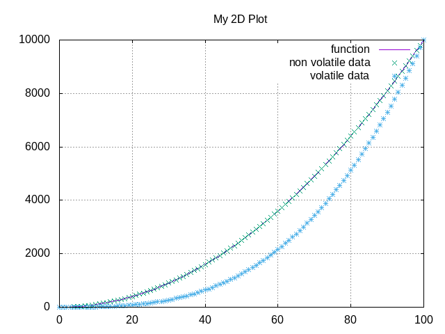
Note that plotting data in this way has some limitations: if there are curves plotted from volatile data it is not possible to plot other curves or functions on the same plot window using the replot option. So if you want to mix on the same plot window volatile curves (i.e. curves plotted using the volatile argument) together with non volatile ones or functions, you must plot the volatile curves as the last plot instruction. Example:

>>> x = numpy.linspace(0,100,101)
>>> y = x * x
>>> z = y * x / 100
>>> gm.plot_function(myplot2d, 'x**2','function')
>>> gm.plot2d(myplot2d, x, y, label='non volatile data', replot=True)
>>> gm.plot2d(myplot2d, x, z, label='volatile data', volatile=True, replot=True)

Note that if there are volatile data are plotted on a plot window, gnuplot does not allow to toggle logarithmic scales on it.

Plotting mathematical functions

Plotting a mathematical expression

If you have not opened a 2D plot window yet (e.g. because you have jumped to this section from the index), you should do it now, using the new_plot() function described in the Creating a new plot window section:

>>> myplot2d = gm.new_plot(plot_type='2D', title='My 2D Plot')

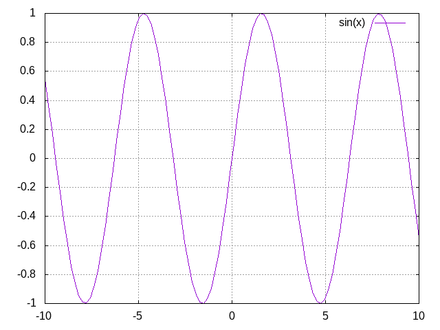
The function plot_function() allows to pass to gnuplot a string, representing a mathematical function [4]:

>>> gm.plot_function(myplot2d, 'sin(x)', label='sin(x)')
(0, 'Ok')

[4]

No check is made that the string represents a valid mathematical expression. If it is not, gnuplot will print an error message on the console or on the file on which you have redirected /dev/stderr (unless you have chosen to send it to /dev/null).

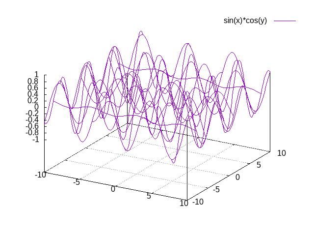
To plot a 3D function, you must open a 3D plot window, if you don’t have done it yet:

>>> myplot3d = gm.new_plot(plot_type='3D', title='My 3D Plot')

>>> gm.plot_function(myplot3d, 'sin(x)*cos(y)', label='sin(x)*cos(y)')
(0, 'Ok')

If the label argument is not given or is set to None, gnuplot will automatically use the function string as a label for the plot legend. If you don’t want any label to be shown, pass the argument label=”” (empty string).

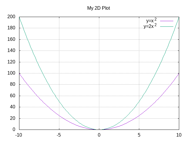
Adding a mathematical expression

By default, plot_function() removes anything that was previously plotted on the window. You can use the replot=True option to plot the function on top of what was plotted before

>>> gm.plot_function(myplot2d, 'x*x', label='y=x^2')
(0, 'Ok')
>>> gm.plot_function(myplot2d, '2*x*x', label='y=2x^2', replot=True)
(0, 'Ok')

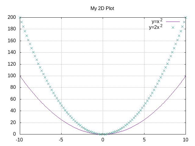
Plotting several mathematical expressions

The function plot_functions() allows to plot an arbitrary number of mathematical expression in a single plot operation, and allows to give a string with additional gnuplot options for each of them.

The expression to be plotted must be recorded in a list, each element of which is itself a list of 3 strings:

• the first one is the math expression;

• the second is the label to be shown on the plot legend;

• the third contains additional options you want to give to gnuplot, [5] or None if you do not want to give them.

[5]

note that no check is made that the string contains valid gnuplot options.

>>> list2d = [ ['x*x', 'y=x^2', 'with lines'],  ['2*x*x', 'y=2x^2','with points'] ]
>>> gm.plot_functions(myplot2d, list2d)
(0, 'Ok')

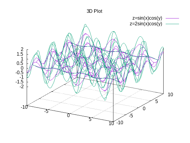
>>> list3d = [ ['sin(x)*cos(y)', 'z=sin(x)cos(y)', None], ['2*sin(x)*cos(y)', 'z=2sin(x)cos(y)', None] ]
>>> gm.plot_functions(myplot3d, list3d)
(0, 'Ok')

If you don’t want to set labels manually, put None in their place and gnuplot will automatically create them, or put “” (empty string) and no label will be shown.

You can pass the replot=True argument to plot functions without deleting anything was plotted before.

A single math expression can be plotted also, with the possibility to give additional options to gnuplot (remember double square brackets):

>>> gm.plot_functions(myplot2d, [ ['x*x', 'y=x^2', 'with linespoints'] ])
(0, 'Ok')

Checking window properties

Printing information on a plot window

The plot_check() function prints information about the plot window given as argument:

>>> myplot = gm.new_plot(plot_type='2D', title='2D plot')
>>> x = numpy.linspace(0,100,101)
>>> y = x * x
>>> z = y * x / 100
>>> gm.plot2d(myplot, x, y, label='y=x^2')
(0, 'Ok')
>>> gm.plot_function(myplot, 'x**2', replot=True)
(0, 'Ok')
>>> gm.plot2d(myplot, x, z, label='y=x^3/100', volatile=True, replot=True)
(0, 'Ok')
>>> gm.plot_check(myplot)
Window index:         0
Window number:        0
Terminal type:        "x11"
Persistence:          "False"
Purge:                "True"
Window type:          "2D"
Window title:         "2D plot"
Number of functions:  1
Number of curves:     1
Number of volatiles:  1
X-axis range:         [None,None]
Y-axis range:         [None,None]
(0, 'Ok')

If the expanded=True argument is given, it prints more information, including the PID of the gnuplot process and the names of the datafiles:

>>> gm.plot_check(myplot, expanded=True)
Window index:         0
Window number:        0
Terminal type:        "x11"
Persistence:          "False"
Purge:                "True"
Window type:          "2D"
Window title:         "2D plot"
Number of functions:  1
Number of curves:     1
Number of volatiles:  1
X-axis range:         [None,None]
Y-axis range:         [None,None]
Gnuplot process PID:  58937
Gnuplot output file:  "/dev/stdout"
Gnuplot errors file:  "/dev/stderr"
Functions
#  0: "x**2"
Curves
#  0: "gnuplot.out/data/gnuplot_data_w0_2D(2D plot)_c0(y=x^2).csv"
(0,'Ok')

Note

Window index is the index of the plot window inside the global variable window_list, while Window number is a unique number attributed to the plot window when it is created, which is used mainly to generate unique names for the data files. The former may change [6], while the latter is fixed for the plot window life.

[6]

As an example, if the first window in window_list is closed, being removed from the list and causing a shift of the indexes.

The function takes two more arguments:

printout (default is True):

if set to True, the output is printed on /dev/stdout/

getstring (default is False):

if set to True, a string with the output is returned. This can be useful to write the output to a file or inside a GUI window.

Printing information on all plot windows

The plot_list() function prints the same information given by the plot_check() function, for all the open windows.

Closing plot windows

Closing a single plot window

When you do not need a plot window anymore, you can close it by means of the plot_close() function, which performs the following actions:

• terminates the gnuplot process associated to the _PlotWindow instance given as argument, by sending the quit gnuplot command to it;

• sets the plot_type attribute of the _PlotWindow instance to None;

• removes the _PlotWindow instance from the window_list global variable.

Note

Closing the window on the screen by clicking on its close button, does not close the gnuplot terminal and does not remove the _PlotWindow instance from the list.

The name given to the _PlotWindow instance (e.g. myplot) is not removed from the namespace. However, if you try to pass it to any function of the package, an error message is returned:

>>> gm.plot_close(myplot2d)
(0. 'Ok')
>>> gm.plot_function(myplot2d, 'x**2')
(11, 'trying to operate on a closed plot window')

Effects of removing plot window names

Note that if you create a plot window with a name (e.g. myplot) and then a second one with the same name, the first one is still in memory (and the associated gnuplot process is still active), but is not linked to that name (myplot) anymore. Example:

>>> myplot = gm.new_plot()
>>> myplot = gm.new_plot(plot_type='3D')
>>> gm.plot_list()
Window index:         0
Window number:        0
Terminal type:        "x11"
Persistence:          "False"
Purge:                "True"
Window type:          "2D"
Window title:         "None"
Number of functions:  0
Number of curves:     0
Number of volatiles:  0
X-axis range:         [None,None]
Y-axis range:         [None,None]

Window index:         1
Window number:        1
Terminal type:        "x11"
Persistence:          "False"
Purge:                "True"
Window type:          "3D"
Window title:         "None"
Number of functions:  0
Number of curves:     0
Number of volatiles:  0
X-axis range:         [None,None]
Y-axis range:         [None,None]
Z-axis range:         [None,None]
(0, 'Ok')

Here we have used the plot_list() function, which is described in the Checking window properties section, to list all the open windows. Now we have two plot windows, one 2D and one 3D, but only the second one is linked to the name myplot, while the first one is not linked anymore to any name. However, the first window is still present in the window_list global variable, so it is shown in the list of windows.

Similarly, if you remove the plot window name from the namespace (e.g. by the del command) without having called the plot_close() function before, the associated _PlotWindow instance and its gnuplot process are not closed, and are still present in the window_list variable. Example:

>>> myplot = gm.new_plot()
>>> gm.plot_check(myplot)
Window index:         0
Window number:        0
Terminal type:        "x11"
Persistence:          "False"
Purge:                "True"
Window type:          "2D"
Window title:         "None"
Number of functions:  0
Number of curves:     0
Number of volatiles:  0
X-axis range:         [None,None]
Y-axis range:         [None,None]
(0, 'Ok')

>>> del myplot
>>> gm.plot_check(myplot)
Traceback (most recent call last):
  File "<stdin>", line 1, in <module>
NameError: name 'myplot' is not defined

>>> gm.plot_list()
Window index:         0
Window number:        0
Terminal type:        "x11"
Persistence:          "False"
Purge:                "True"
Window type:          "2D"
Window title:         "None"
Number of functions:  0
Number of curves:     0
Number of volatiles:  0
X-axis range:         [None,None]
Y-axis range:         [None,None]
(0, 'Ok')

After deleting the myplot name, it is not possible to check the plot window by plot_check(myplot), because the window is not anymore linked to that name. However, we can still check the plot window using the plot_list() function, since it relies on the content of the window_list global variable, which was not altered by the del command. It is also still possible to reference the window as window_list[index], where index is the window index given in the output of the plot_list() function.

You could also create a plot window (i.e. a _PlotWindow instance) without giving a name to it:

>>> x = linspace(0,100,101)
>>> gm.plot1d(gm.new_plot(),x)

in this way, the plot window is created and passed directly as argument to the plot function (plot1d() in this example) without giving a name to it. Also in this case, the newly created plot window will appear in the output of the plot_list() function.

The plot_close_all() function, described in the Closing all the open windows at once paragraph, closes all the plot windows (and terminates their associated gnuplot processes), including the ones which are not linked to any name.

Deleting the output files

When a plot window is closed, the data files associated to the curves are deleted or not, depending on the value of its purge attribute, which was set when the plot window was opened according to the value of the purge argument passed to the new_plot() function. Examples:

>>> myplot = gm.new_plot(purge=True)

the datafiles will be deleted each time new data is plotted (without giving the replot=True argument) and when the window is closed;

>>> myplot = gm.new_plot(purge=False)

the datafiles will not be deleted each time new data is plotted and not be deleted when the window is closed.

The default behavior is stored in the PURGE_DATA global variable:

>>> print(gm.PURGE_DATA)
True

If the plot was opened passing the redirect_output=True argument, the files on which the gnuplot output and errors have been redirected are deleted or not in the same way. If you want to preserve them, when the the window has the purge option active, you can pass the keep_output=True argument to the plot_close() function.

The optional delay parameter specifies a time (in seconds) to wait before deleting the data files, after the quit command has been sent to gnuplot. This can be useful in some circumstances, for example if you want to create a persistent window, plot something complex on it, and then close the gnuplot process leaving only the window open:

>>> myplot = gm.new_plot(persistence=True, purge=True)
>>> x = numpy.linspace(0, 1000, 1000000)
>>> y = x * x
>>> gm.plot2d(myplot, x, y)
(0, 'Ok')
>>> gm.plot_close(myplot, delay=1)
(0, 'Ok')

When the plot_close() function is called, it immediately sends the quit command to gnuplot, but it is executed only when gnuplot has completed the plot operation started by the plot2d() function. If the datafiles were deleted immediately after sending the quit command, they could be removed while the plot operation (plotting one million points) is still in progress.

Closing all the open windows at once

The plot_close_all() function closes all the plot windows listed in the window_list global variable, and empties it. It works calling the plot_close() function, so it gets the same arguments.

>>> gm.plot_close_all()
(0, 'Ok')

By default, the function tries to delete the gnuplot.out directory, if it is empty. If you don’t want to delete it, you can pass the purge_dir=False argument.

Performing other actions

Changing the window properties

You can change some properties of a plot window, such as logarithmic scale or range of the axes, using the plot_set() function. Example, to set logarithmic x axis:

>>> myplot = gm.new_plot(logx=False)
>>> gm.plot_set(myplot, logx=True)   # I have changed my mind...
(0, 'Ok')

By default, the new options are applied when a new curve or function is plotted: if you want to apply them immediately, on the already plotted items, pass the replot=True argument:

>>> x = numpy.linspace(1, 100, 100)
>>> y = numpy.exp(x)
>>> gm.plot2d(myplot, x, y)
(0, 'Ok')
>>> gm.plot_set(myplot, logx=False, logy=True, replot=True)
(0, 'Ok')

To know which settings are available, read the function docstring:

>>> help(gm.plot_set)

Only a few of the many possible settings provided by gnuplot are implemented in this function. However, you can use the plot_command() function to send to gnuplot any command you wish, as described in the section Sending arbitrary commands to gnuplot.

Refreshing windows

You can refresh the plot window at any time using the plot_replot() function:

>>> gm.plot_replot(myplot)
(0, 'Ok')

If you have closed the window by clicking on its close button, this will cause it to reappear.

You can refresh all plot windows at once by the plot_replot_all() function:

>>> gm.plot_replot_all()
(0, 'Ok')

Resetting windows

The plot_reset() function allows to reset the window properties:

• removes all the curves and functions

• clears the plot area

The plot_axes argument, which is True by default, tells the function to plot the axes [7] after having cleared the window.

If one axis has a defined range which is completely negative (e.g. [-2,-1]) and the logarithmic scale has been set, the linear scale is restored since it would be impossible to plot any data.

[7]

to force gnuplot draw the axis, a small dot is plotted, which is barely visible, and is automatically removed as soon as something is plotted on the window.

The plot_reset_all() function resets all the plot windows at once.

Printing a label on the plot window

You can print an arbitrary string on the plot window using the plot_label() function

>>> myplot = gm.new_plot()
>>> gm.plot_label(myplot, x=10, y=10, label='This is a parabola !', erase=False)
(0, 'Ok')
>>> gm.plot_function(myplot,'x**2')
(0, 'Ok')

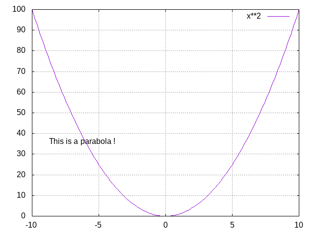
x and y give the position at which the string must be printed, expressed in characters, starting from the lower-left angle (x=1,y=1) of the graph. The erase=True argument removes all previously printed strings before printing this one. If you pass the erase=True, but don’t pass the label argument, the plot is cleared from previously printed labels:

>>> gm.plot_label(myplot, erase=True)
(0, 'Ok')

By default, the label is not printed immediately, but is shown when a new curve of function is plotted. If you want the label to be shown immediately, you can pass the replot=True argument. However, it will work only if some plots or curves have been plotted before (and therefore can be replotted).

>>> gm.plot_label(myplot, x=50, y=20, label='Hello !', erase=False, replot=True)
(0, 'Ok')

Read the function docstring for more details:

>>> help(gm.plot_label)

Exporting a plot window to a file

A plot can be exported to a file in various formats using the plot_print() function. The first argument passed must be the _PlotWindow instance of the plot you want to export, followed by the following optional arguments:

• the terminal used to create the image;

• the directory in which file must be saved (default is the CWD);

• the filename;

• an optional string with additional options to pass to gnuplot.

Example:

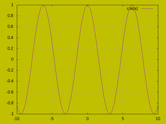
>>> myplot = gm.new_plot()
>>> gm.plot_function(myplot, 'cos(x)')
(0,'Ok')
>>> gm.plot_print(myplot, terminal='png', dirname='images', filename='cosx.png', options='background \"#c0c000\"')
(0, 'Ok')

The file cosx.png is saved in the images directory, which is created in the current working directory if it doesn’t exist yet, with the following image:

If the filename is not given, a default name is given to the output file, in the form:

output_window#<n>.<ext>

• <n> is the window number (window_number attribute of the _PlotWindow instance)

• <ext> is a standard extension depending on the terminal, (e.g. ‘.png’ for png terminal).

The default terminal is stored in the global variable DEFAULT_PRINT_TERM, while the list of allowed terminals is stored in PRINT_TERMINALS:

>>> print(gm.DEFAULT_PRINT_TERM)
png
>>> print(gm.PRINT_TERMINALS)
('png', 'jpeg', 'eps', 'gif', 'svg', 'latex', 'postscript', 'pdfcairo', 'dumb')

Read the function docstring for more details:

>>> help(gm.plot_print)

Exporting all the plot windows

You can also export all the open plot windows at once, using the plot_print_all() function. In this case, however, the default filenames are used, and the options, if given, are the same for all the windows. You can still pass the argument dirname to select a directory where all the files must be saved. Example:

>>> gm.plot_print_all(dirname='images')

all the open plots will be saved in the images directory, which will be created if it doesn’t exist yet.

Sending arbitrary commands to gnuplot

You can send arbitrary commands to the gnuplot process associated to a plot window using the plot_command() function:

>>> myplot=gm.new_plot()
>>> gm.plot_command(myplot,string='<gnuplot-command>')

Note

No check is made that the string you provide is a valid gnuplot command: if it is not, gnuplot rises an error, which can be printed on console, written to file, or discarted, depending on the value given to the redirect_output parameter when the function new_plot() was called to create the plot.

List of available functions

Read the doctrings for a complete description of each function.

Create, modify, and close plot windows

new_plot()

create a new plot window

plot_set()

modify some properties of a previously created window

plot_command()

send a command to the gnuplot process

plot_close()

close the plot window and terminate the gnuplot process

plot_close_all()

close all the plot windows and terminate all the gnuplot processes

Plot data

plot1d()

plot a curve from 1d data

plot2d()

plot a curve from 2d data

plot3d()

plot a curve from 3d data

plot_box()

plot a boxplot from 1d data

plot_curves()

plot several curves at the same time

Plot mathematical functions

plot_function()

plot a mathematical expression

plot_functions()

plot several mathematical expression at once

Print plots to files

plot_print()

export a plot to a file

plot_print_all()

export to files all the open plots

Reset, clear and refresh plots

plot_reset()

reset a plot: remove all curves and functions and the clear the window

plot_reset_all()

reset all plot windows

plot_clear()

clear the plot area

plot_clear_all()

clear the plot area of all plots

plot_replot()

refresh the plot window

plot_replot_all()

refresh all the plot windows

Utility functions

plot_label()

print a string on the plot

plot_raise()

rise the plot window over the other windows on the screen

plot_lower()

lower the plot window under the other windows on the screen

plot_raise_all()

rise all the plot windows

plot_lower_all()

lower all the plot windows

plot_check()

print the plot properties

plot_list()

print the properties of all plots

The _PlotWindow class

Each plot window is an instance of the _PlotWindow class, which has several attributes:

self.window_number:

an integer number that identifies the plot window, [8] mainly used to generate unique names for the data files

self.gnuplot_process:

gnuplot process (instance of subprocess.Popen)

self.term_type:

the type of gnuplot terminal

self.plot_type:

a string defining the type of plot : ‘2D’, ‘3D’, or None if the plot window has been closed

self.n_axes:

number of plot axes (2 for 2D plots, 3 for 3D ones)

self.xmin:

minimum of the x-axis (None if not set)

self.xmax:

maximum of the x-axis (None if not set)

self.ymin:

minimum of the y-axis (None if not set)

self.ymax:

maximum of the y-axis (None if not set)

self.zmin:

minimum of the z-axis (None if not set)

self.zmax:

maximum of the z-axis (None if not set)

self.persistence:

True if the plot was opened as persistent

self.title:

the window title (None if not given)

self.filename_out:

name of the file to which gnuplot output is redirected

self.filename_err:

name of the file to which gnuplot errors are redirected

self.data_filenames:

list containing the names of the datafiles related to the curves presently plotted on the window

self.n_volatiles:

number of curves that have been plotted using the volatile=True argument: they are not listed in self.data_filenames since there are no associated data files

self.functions:

list containing the function strings [9]

slef.purge:

if True, old data files are removed when new data is plotted without the replot=True option or when the window is closed

self.error:

if there was an error while creating the plot window, an error message is stored here

[8]

Note that this number is not the index that identifies the plot window inside the window_list variable: in fact the former is fixed, while the latter may change when other windows are removed from the list.

[9]

Note that no check is made that function strings given to gnuplot are correct. So even wrong ones (which therefore gnuplot has not plotted) are listed here.

Note

If you modify the plot by sending commands to gnuplot directly, using the plot_command() function, some of these attributes, such as the number of curves and the list of data files, may not be updated properly.

The _PlotWindow class have some methods also, which are called by the functions of the functions.py module to perform their tasks:

self._command()

method used to send commands to gnuplot

self._quit_gnuplot()

method used to terminate the gnuplot process and close the window

self._add_functions()

method used to add one or more mathematical expression

self._add_curves()

method used to add one or more curves from data

Note

Since the package is designed to use the functions in the functions.py module, these methods are not intended to be called directly.