
GP_ELITE
Genetic-programming symbolic regression — discover interpretable laws from your experimental data.
Declare your units and the search only ever builds dimensionally valid equations — a hard constraint, not a soft penalty. The operating envelope is measured, not claimed: how many points it needs, how its runtime grows, and where it fails.
🇫🇷 Version française

GP_ELITE searches for a mathematical formula linking your variables to a target, instead of a black box. It is built for small experimental datasets (≤10 variables) where you want to understand the relationship: degradation laws, sensor calibration, engineering correlations, dose-response curves, physical laws.
On five Feynman equations (without normalisation), the returned model recovers the exact law of four of them at every size from 25 to 10,000 points, in every run; the fifth, the nested rational form I.16.6, is not recovered exactly at any size. The five fits take 108 s in total at 1,000 points and 284 s at 10,000 (benchmarks/feynman_scaling.py, version 0.8.0).
Since 0.4 "Lawful" you can also declare the physical units of your columns — the search itself then only ever builds dimensionally sound expressions, instead of formulas that fit the numbers while breaking the physics (see Dimensional constraints below).
Pure Python / NumPy — no Julia, no compilation, no GPU. pip install and you're ready.
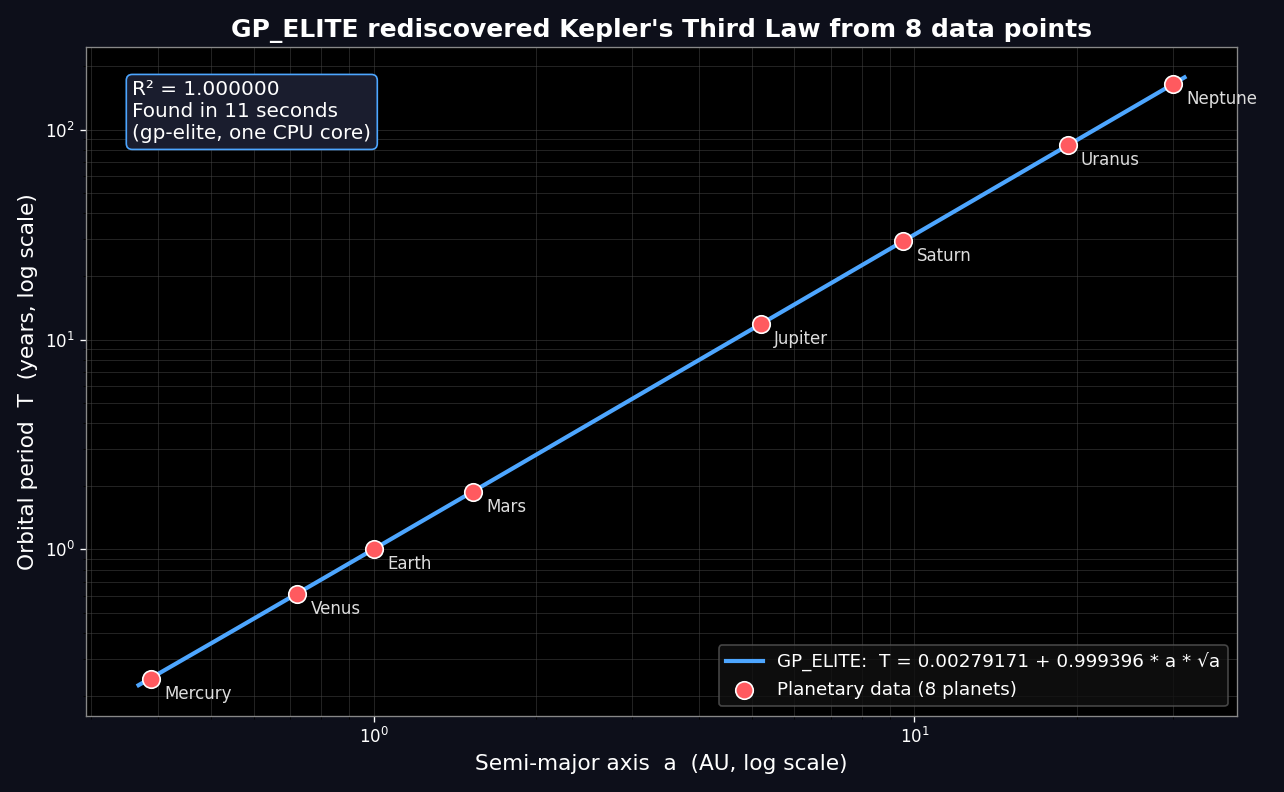
Given only the 8 planets' distance and orbital period, GP_ELITE rediscovered Kepler's Third Law,
T = a·√a = a^1.5— seeexamples/kepler_demo.py.
import numpy as np
from gp_elite import symbolic_regression

a = np.array([0.387, 0.723, 1.000, 1.524, 5.203, 9.537, 19.191, 30.069])   # AU
T = np.array([0.241, 0.615, 1.000, 1.881, 11.862, 29.457, 84.011, 164.79])  # years

result = symbolic_regression(a.reshape(-1, 1), T, feature_names=["a"], generations=40, seed=0)
print(result.expression)     # 0.00279171 + 0.999396 * a * sqrt(a)
The formula is written in your variables and units: in astronomical units and years, Kepler's constant is 1, and that is what comes back.
Is this for you?
You probably want GP_ELITE if at least one of these is true:
- You have a table of measurements and want the formula, not a prediction. A degradation curve, a sensor calibration, an engineering correlation. You care about the shape of the relationship, and you intend to read it, sanity-check it, maybe publish it.
- You cannot install a second language runtime. A locked-down university
machine, a corporate laptop without admin rights, a CI container you do not
control.
pip install gp-eliteand its three dependencies are all you need — no compiler, no Julia, no GPU. - You know the physical units of your columns. Declare them and the search will only ever build dimensionally sound formulas — and can tell you the units and value of a physical constant that is not in your data at all.
- You are teaching or learning genetic programming. The engine is plain Python you can read, step through and modify, and it ships with an interactive console that needs no code at all.
If none of these fit, other tools may serve you better: PySR and Operon are
faster and more accurate at scale — see Is it solid? below.
Installation
pip install gp-elite          # from PyPI
# or, from source:
git clone https://github.com/ariel95500-create/gp-elite
cd gp-elite && pip install -e ".[test]"
Dependencies: numpy, pandas, scikit-learn. Python 3.9 to 3.14, tested on Linux and Windows.
Usage
One line, on your own data (console UI)
gp-elite
Choose mode 6 (generic CSV), point to your file, and keep the defaults. GP_ELITE detects the columns, holds out a validation set, evolves, and prints the discovered law — written in your own column names and units, checked against its own predictions on your data.
Mode 6 also asks for the physical units of your columns. Declaring them is optional, and skipping is one keystroke — but if you do declare them, the search is restricted to dimensionally consistent formulas, and the engine can deduce the units and value of a missing physical constant. On a two-column CSV of Hooke's law it returns:
  Units for ['elongation'], comma-separated : m
  Unit for TARGET 'force' : N
  Deduce an unknown constant? [y/N] : y
  ...
  Formula in YOUR columns (checked on your data):
    force = 250 * elongation
  Deduced constant units : [kg / s^2]
  Deduced constant value : 250
Programmatically (notebooks, pipelines)
import numpy as np
from gp_elite import symbolic_regression

rng = np.random.RandomState(0)
X = rng.uniform(1, 5, (200, 2))
y = 2.0 + 3.0 * np.sqrt(X[:, 0]) - 0.5 * X[:, 1]

if __name__ == "__main__":        # needed in scripts, see the note below
    result = symbolic_regression(
        X, y,
        feature_names=["a", "b"],
        operators="physical",     # 'physical' | 'trig' | 'full' | 'poly' | 'conserve'
        generations=60,
        speed="fast",             # 'ultrafast' | 'fast' | 'normal' | 'thorough'
        seed=0,
    )
    print(result.expression)      # 2 + 3 * sqrt(a) - 0.5 * b
    print(result.r2_validation)   # 1.0
    print(result.size)            # 33 (nodes of the engine's tree)
    print(result.sympy())         # the same formula, parsable by sympy
Here the search returns the law it was given, written in your variables: the
engine's tree has 33 nodes, and the formula printed from it is 2 + 3·√a − 0.5·b;
the fit checks that this formula reproduces predict(). That is not guaranteed. On a harder law the same budget returns an
approximation that fits the hold-out almost perfectly and is still not the law
(0.7 returned one for this very example); reading the formula is how you find out.
restarts= and speed="thorough" spend more compute on the exact form, without a
guarantee.
speed:'ultrafast' | 'fast' (default) | 'normal' | 'thorough'.'thorough'(population 400, four islands, 200 generations) is the regime for looking for an exact law; with twice the default number of generations, it is slower, and not guaranteed to do better.time_limit=(seconds): the search stops cleanly at the deadline and returns the best model found so far, instead of being killed without a result; the final selection that follows adds a little (under two seconds for a 15 s budget in our measurement: 16.7 s on 3,000 rows).restarts=: independent evolutions whose candidates are merged before the final choice.
Your data. X can be a NumPy array, a list of rows or a pandas DataFrame,
whose column names then become the variable names; y a 1-D array or a single
column. A missing or infinite value is refused with the row and the column
concerned (remove or impute it first), and a non-numeric column is named in the
error. With 0.7, a missing value in y or in a column the law uses went through,
and the fit returned an unrelated formula without a warning
(benchmarks/bad_input_check.py). Values far from 1 need no preparation: a
target of order 1e-9 or 1e20 is divided internally by a power of ten, a column of
order 1e-19 by its largest absolute value (the default normalisation), and the
formula comes back in your units (up to 0.7, such a target returned a constant or
a wrong line, with a negative R², and no warning that the fit had failed).
Reproducibility. With the same seed, the same data and the same settings, a
fit returns the same model, run after run, without setting PYTHONHASHSEED
(required up to 0.7). Parallel islands follow another path than the sequential
search, and parallel=None turns them on from four cores: set parallel= too
to get the same model on another machine.
Scripts and parallel islands. On machines with four cores or more, islands run
in parallel worker processes. Those workers are started with spawn on every
system (Linux included) and re-import your script, so keep the top-level code
under if __name__ == "__main__":, as above.
Without the guard GP_ELITE detects the situation, finishes on one core with the
same result, and says so once. Notebooks need nothing.
Reading the result
expressionis written in your variables. The engine searches on rescaled columns internally; the formula it returns has the rescaling folded back into its constants, and the fit checks that the formula reproducespredict()on your data (result.formula_exact).result.sympy()gives the same formula as a stringsympy.sympifycan parse, andresult.sympy_expr()the sympy expression itself, with one symbol per column: use it when a column name is also a sympy constant or function (sympifyreadsEas 2.718...,Ias √-1) or is not an identifier;sympy()warns in that case. (Before 0.7, the displayed constants were those of the internal scaled space.) The formula is the plain mathematical function: where one of the engine's numerical safety nets acts on your data (a power clipped because its base exceeds 100 or its exponent 6 in absolute value, or its value a million; a division by a denominator within 1e-8 of zero), or, rarely, where rounding ruins an ill-conditioned expression, it departs frompredict()on those rows,formula_exactis False and the fit warns. In the measurements of 0.8 (benchmarks/results_0.8/), that was the case for 6 of the 205 Feynman fits of the release at 30 s per fit, for none of 60 fits on standardised real data and 8 of 70 on real data in their own units (campaigns 5b and 6b), and for 1 of the 105 fits of the equal-work comparison (100 generations).r2_validationis a selection score. The hold-out it is computed on is also used to choose the returned model among the candidates, so it is optimistic. To estimate how the formula generalises, keep a test set of your own out of the fit.result.paretolists the other non-dominated candidates, simplest first, each with its ownexpression,r2_validationandpredict.predict()checks what it is given. It expects as many columns as the fit had (a single sample isX.reshape(1, -1)), and returns NaN for a row with a missing or infinite input, where 0.7 returned 0.
🛡️ Robust regression (outlier-resistant custom loss)
Real-world data is dirty. A handful of outliers can drag an ordinary least-squares fit far from the true relationship. GP_ELITE ships a one-switch robust mode meant to follow the bulk of the data rather than a few extreme points.
result = symbolic_regression(X, y, feature_names=["x"], robust=True)
Under the hood, robust=True switches the objective to a Huber loss and rescales the final coefficients with an IRLS (Iteratively Reweighted Least Squares) procedure. It stays a compact, readable formula.
Measured behaviour (recovering y = 2x + 1; RMSE against the true law on the clean points, lower is better; five seeds, median and worst seed):
| outliers | default (MSE) | robust=True |
|---|---|---|
| 0 % | 0.063 [0.063] | 0.063 [0.063] |
| 10 % | 1.398 [1.398] | 0.237 [0.237] |
| 20 % | 1.925 [1.925] | 1.925 [1.925] |
On clean data the two modes return slightly different lines, equally close to the true
law. With 10 % outliers, robust mode cuts the error six-fold. With 20 %, on this
example, it does no better than the default: the default returns the same line for all
five seeds, pulled by the outliers (y = 4.23319 + 1.32825 * x), and robust mode the same
line for four seeds out of five. Robustness is a tool to try when you suspect outliers,
not a guarantee — compare both modes on data of your own.
(Up to 0.6 this table reported the best of three runs, picked by comparing with the
true law, which no user can do.)
Reproduce: python examples/robust_regression.py.
⚖️ Dimensional constraints (physical laws only)
Declare the units of your inputs and target, and GP_ELITE will only search expressions that are dimensionally sound — no more formulas that fit the numbers while being physically meaningless.
from gp_elite import GPEliteRegressor

est = GPEliteRegressor(
    units=["kg", "m/s"],      # units of X0, X1
    target_units="J",         # unit of the target
)
est.fit(X, y)
Units accept plain strings — SI bases (m kg s A K mol cd), common derived units
(N J W Pa Hz C V ohm T), and * / ^ ( ): "m/s", "kg*m/s^2", "s^-1",
"1" for dimensionless. Dimension dicts ({"m": 1, "s": -1}) work too, as do
per-name ({"X0": "kg"}) and per-index ({0: "kg"}) forms. A malformed string
("m/(s", "kg^", "m garbage") raises an error instead of being guessed.
Measured effect — Feynman II.11.3, x = q·Ef/(m·(w0²−w²)), 5 variables,
5 seeds, 40 generations, identical budget for the first two arms:
no units= |
units= |
no units=, 4x generations |
|
|---|---|---|---|
| dimensionally valid | 0 / 5 | 5 / 5 | 0 / 5 |
| exact law recovered (holds out of domain) | 0 / 5 | 2 / 5 | 0 / 5 |
| median test R² | 0.99157 | 0.99957 | 0.99863 |
| median out-of-domain R² | 0.34 | 0.65 | 0.42 |
| median model size | 59 nodes | 27 nodes | 60 nodes |
| median seconds / run | 21 | 149 | 84 |
The third column gives the unconstrained arm four times the generations. It still
yields 0/5 physically valid models: compute does not substitute for the
constraint. (The constrained search is the slower one, and slower than with 0.7,
which took 57 s: a search now stops early only on an exact law, so the constrained
runs that end on an approximation go through all 40 generations, although each
generation takes about a fifth less time than with 0.7 (two seeds, run side by
side). time_limit= bounds it.)
The unconstrained failures are not marginal: across the ten unconstrained runs, the
models take the logarithm of a frequency or of another quantity with units, add
kilograms or hertz to pure numbers, or raise a quantity to an exponent in coulombs
or in hertz.
What it does not do. On a test set drawn outside the training domain (w/w0
pushed from [0.20, 0.67] towards resonance at [0.70, 0.90]), approximations degrade
in every arm. Two constrained runs in five found the exact law, which holds there
(R² = 1.00000); the other three are physically coherent approximations, not the law. Timings are from a 2-core Linux container, one run per core. Reproduce with
benchmarks/ab_ood.py.
When to use it. For discovering physical laws when you know the units and the law is dimensionally homogeneous, and to guarantee that whatever the engine returns is at least physically meaningful. Not for black-box prediction: the constraint rules out dimensionally wrong but numerically good approximations, so it can lower R² when fitting is the goal rather than finding a law.
Laws with a dimensioned constant (unknown_constant=). By default, fitted
constants are dimensionless — the AI Feynman convention — which puts a law like
Hooke's F = k·x out of reach: no dimensionless constant can relate metres to
newtons, and the search correctly reports that nothing valid can be built. Set
unknown_constant=True and the leading constant is allowed to carry a
dimension, deduced by homogeneity:
est = GPEliteRegressor(units=["m"], target_units="N", unknown_constant=True)
est.fit(X, y)
est.constant_units_string()   # '[kg / s^2]'
est.constant_value_           # 250.0
The engine then reports not only the shape of the law but the units and value of the missing physical constant. Measured on three reference laws:
| law | structure recovered | deduced units | value | true |
|---|---|---|---|---|
Hooke F = k·x |
yes | kg / s² |
250 | 250 |
Newton F = G·m₁·m₂/r² |
yes | m³ / kg s² |
6.674e-11 | 6.674e-11 |
ideal gas P = nRT/V |
yes | kg m² / K mol s² |
8.314462618 | 8.314462618 |
The returned formula itself carries the physical constant: the benchmark prints
(250.0*X0) for Hooke and (8.314462617999999*((X0*X1)/X2)) for the ideal gas.
Budget: 25 generations, two restarts.
Reproduce with benchmarks/test_constante_mystere.py. Requires units= and
target_units=. If the expression is not a monomial in the input columns
(m₁ + m₂, say), no single raw constant exists and constant_value_ is None
while the deduced units remain valid.
Limitation. Under units= the internal linear scaling is multiplicative
only (no additive offset), which keeps every candidate dimensionally homogeneous.
Example on simulated battery-ageing data
python examples/battery_soh.py
The file examples/nasa_battery_simulation.csv
holds 168 simulated charge cycles (cycle number, temperature, current, capacity
state of health). Its origin is not documented beyond its name, so treat this as a
demonstration of the workflow, not as a result on real batteries. On it, the script
prints (abridged):
PROTOCOL 1 — random split (INTERPOLATION, leaks info)
  GP_ELITE      R² = +0.991
  RandomForest  R² = +0.997
  XGBoost       R² = +0.997

PROTOCOL 2 — forward split (EXTRAPOLATION): train on cycles 1..142, predict 143..168
  RandomForest (300)      R² = -2.515
  XGBoost (300 trees)     R² = -2.324
  GP_ELITE (one equation) R² = -0.314

  Equation: SOH = 0.413666 + 0.500082 * tanh(2.40159 * temperature / cycle)
A random split of sequential data is interpolation and flatters every method. On the forward split, the tree ensembles can only repeat values seen in training and fall far below the mean. The equation found by 0.8 does better than them but not well (R² −0.31, below the mean too); the one 0.7 found on the same split, in the cycle and the current, kept following the trend (R² +0.594). A formula can extrapolate where a tree ensemble cannot; whether it does depends on which formula the search returns — on this simulated set, to be checked on yours.
Is it solid?
A fair question for a project you have never heard of. Here is where it stands against the alternatives, and where it does not.
| GP_ELITE | Neural networks | PySR (state of the art) | |
|---|---|---|---|
| Output | readable formula | black box | readable formula |
| Installation | pip install (pure Python) |
heavy | requires Julia |
| Held-out validation | built in (used for model selection) | do it yourself | do it yourself |
| Physical units | hard constraint during search (units=) |
no | soft penalty (X_units=) |
| Stability of the answer | bootstrap report (stability_analysis) |
no | no |
| Speed and accuracy at scale | lower | — | higher |
How changes are decided. Since 0.8, a change meant to improve the search or
the final selection becomes part of the default behaviour only if it passes a
comparison written in advance: the hypothesis and the decision criteria are
committed before the first run
(benchmarks/results_0.8/PLAN.md;
the plan of the first campaign was committed six minutes after its first fit had
started), the engine with the change is compared with the engine without it on 41
Feynman equations and on real datasets (six standardised, seven in their own
units) at 30 seconds per fit, one process per fit, and the results are published
whatever they are
(RESULTS.md),
including the changes that did not pass. When a change failed and a restricted
version of it was then tested, the restriction was designed after seeing the
failure and measured on the same problems; RESULTS.md says where. Corrections of
defects are not decided this way; the files of benchmarks/results_0.8/ show what
they change.
GP_ELITE's niche: zero barrier to entry. A lab engineer, a student, or a technician points at a CSV file and gets a validated law back — without becoming a developer. PySR and Operon are faster and more accurate on large or hard problems; GP_ELITE does not claim otherwise.
What is GP_ELITE good (and less good) at?
Good at: physical / engineering laws with multiplicative or exponential structure, modest-size experimental data, problems where interpretability matters most.
On the frozen Feynman benchmark (15 physics equations, restarts=4, one seed),
judged on the model it returns: 12/15 exact symbolic recoveries (1−R² < 1e-9 on
held-out data) and 13/15 within 1e-3; the misses are I.16.6 (relativistic velocity
addition, a nested rational form) and I.18.12 (r·F·sin θ, which 0.7 recovered with the
same budget), and III.15.12 comes back within 1e-3. Head-to-head against gplearn on
identical data and splits (population 2000 × 30 generations), each method judged on
its returned model: 12/15 against 6/15 exact, 13/15 against 7/15 within 1e-3 —
GP_ELITE ahead on 8 equations, tied on 6, behind on one (I.18.12). Without the column
normalisation (normalize='none', same budget), the three laws with a sine or a
cosine all come back exact, I.18.12 and III.15.12 included
(python benchmarks/feynman_bench.py 12 15 --normalize none). With the physical
units declared (units=, same budget, no normalisation), 14/15 come back exact, each
in its textbook form (benchmarks/feynman_units.py). One seed on fifteen equations is
a showcase, not a statistical comparison:
benchmarks/results_0.8/RESULTS.md
measures 0.7.0 and each change of 0.8 to the search and the final selection on 41
equations with five seeds at 30 s per fit, and 0.7.0 against 0.8.0 side by side at
equal work on these fifteen equations with five seeds and on six real datasets.
Reproduce: python benchmarks/feynman_bench.py 0 15 and python benchmarks/duel.py.
Less good at: chaotic sequences (e.g. Collatz flight time — an intrinsically random component), >15–20 variables (the search space explodes — though units= substantially narrows it when physical units are known), large datasets where raw accuracy outweighs interpretability (ensemble models dominate there).
Technical features
- Power-law seeds (v0.8): when the data follow a power law, the monomial fitted on the logarithms starts in the population
- Exact-law polish (v0.8): finalists get converged constants and a coefficient per term of each sum; a variant is admitted only if it is exact
- Constants fitted for the judged form (v0.8): Levenberg–Marquardt in variable projection (the scale and offset of the linear scaling solved inside the residual)
- Scale-free data (v0.8): a target of any magnitude is divided internally by a power of ten, and the default normalisation divides each column by its largest absolute value
- Formula in your variables, checked (v0.7): the internal rescaling is folded back into the constants;
formula_exactreports whether the formula reproducespredict()on the training data - Time budget (v0.7):
time_limit=stops cleanly and returns the best model found - Mystery-constant deduction (v0.5): the leading constant may carry a dimension, inferred by homogeneity; units and raw value exposed on the estimator
- Dimensionally-constrained search (v0.4): constructive typed generation, dimension-preserving mutation and crossover, validity gate in
fitness()— one semantics shared with the post-hoc auditor (v0.7) - Scale-only linear scaling under
units=(v0.4.1): regression through the origin, so the form that is scored is the form that is delivered - Numerical guard in the LM optimizer (v0.4): no more float64 overflow on unbounded
sq/cube/*chains - Post-hoc dimensional audit (v0.3):
dimensions.py - Levenberg–Marquardt constant optimization (v0.2): deterministic, LM/Adam switchable
- Multi-restart + merged candidate archives (v0.2): seed variance turned into reliability
- Pareto front API (v0.2): non-dominated complexity/accuracy staircase
- Guarded extrapolation / forecasting mode (v0.2): beyond-domain probes, linear floor, frontier selection
- Composition motif seeding (v0.2): Pythagorean, reciprocal-sum, Gaussian templates for nested structures
- Asymmetric island model (explorer / cleaner / stigmergic) with periodic migration, in parallel worker processes on machines with four cores or more
- Linear scaling (Keijzer 2003): the engine searches for the shape; scale and offset are solved in closed form
- ε-lexicase selection (La Cava 2016) to preserve behavioral diversity
- Hold-out validation + parsimonious champion selection (R² tolerance)
- Shift-free normalization preserving multiplicative structure (x·y stays a clean product), for all data since 0.7
- Stigmergic memory exportable across runs (grammar export/import) — a documented feature, not a measured performance advantage
What's new
0.8 "Swift" — faster (the speed-ups alone return the same models), more laws
recovered (power laws seeded, right structures finished into exact laws), data of
any scale, inputs checked; every change meant to improve the search decided by a
comparison written before it ran. 0.7 "Sound" — the formula you get is the model you got: written in your
variables for every normalisation and checked at fit time; a time_limit=
budget; dimensional guarantees made strict; every number of its README
re-measured on its final code. 0.6 "Bench" — physical units in the
console. 0.5 "Unknown" — units and value of a law's missing constant.
0.4 "Lawful" — dimensionally-constrained search. 0.3 "Trust" —
diagnostics and stability.
Full history, with the measurements behind each claim, in
CHANGELOG.md. Every benchmark behind a number here lives in
benchmarks/, with its raw results.
Did it fail on your data? Please say so
GP_ELITE is tuned on published benchmarks — Feynman, Strogatz — which are clean, noise-free and well-scaled. Real measurements are none of those things, and that gap is where the engine most needs work.
So if it returns nonsense on your data, that is useful information, not user error. Open an issue with the shape of your data and what you got back. You do not need to share the data itself, you do not need to know why it failed, and you can write in English or French.
Failure reports on real measurements are the single most valuable contribution this project can receive. See CONTRIBUTING.md.
Tests
pip install -e ".[test]"
python -m pytest tests/ -q
tests/test_guarantees.py pins down every defect found so far — each test was
checked to fail on the code that had the defect. The suite runs on every push
that changes code (Linux, Python 3.9–3.14, and Windows).
License
MIT — see LICENSE. Free to use, including commercially, with retention of the copyright notice.
Citing GP_ELITE
If GP_ELITE is useful in academic work, see CITATION.cff.
1 maintainer

Metadata
1 maintainer
Release files for gp-elite 0.8.0
For a detailed explanation of source distributions (sdists) and built distributions (wheels), please see the package formats documentation.
Source distribution (sdist)
| File | Size | Uploaded | |
|---|---|---|---|
| gp_elite-0.8.0.tar.gz | 244.9 kB | Details |
Built distribution (wheel)
| File | Interpreter | ABI | Platform | Reset |
|---|---|---|---|---|
| gp_elite-0.8.0-py3-none-any.whl | Python 3 | none | any | Details |
Total release size: 457.9 kB
Release files / gp_elite-0.8.0.tar.gz
| Download URL | gp_elite-0.8.0.tar.gz |
|---|---|
| Size | 244.9 kB |
| Tags | Source |
|
SHA-256 checksum How to use checksums |
ba3f4deca46e8a366fa304e129b8dde3e7c740cf5d1cded8f1a3a027e16f6a22
|
|
BLAKE2b-256 checksum How to use checksums |
b661ed39e38ad3ab729d3e6b64277911205e48c616b638cb974b7bc1cf464d9a
|
| Upload date | |
|
Uploaded using Trusted Publishing? What is trusted publishing? |
No |
| Uploaded via |
twine/7.0.0 CPython/3.14.4
|
Release files / gp_elite-0.8.0-py3-none-any.whl
| Download URL | gp_elite-0.8.0-py3-none-any.whl |
|---|---|
| Size | 213.1 kB |
| Tags | Python 3 |
|
SHA-256 checksum How to use checksums |
b0ca029cd0810cbd2faf30353aee185abd19f28995ee70168ce4061be1aaf891
|
|
BLAKE2b-256 checksum How to use checksums |
cd0028bcee75f307ff5f6a04e4f01127deea7afaa2572dcdef22166084b1ba38
|
| Upload date | |
|
Uploaded using Trusted Publishing? What is trusted publishing? |
No |
| Uploaded via |
twine/7.0.0 CPython/3.14.4
|














