
GP-VAR — Gaussian Process Vector Autoregressions with Stochastic Volatility in Python
gpvar is a complete, self-contained Python implementation of the Gaussian process vector autoregression (GP-VAR) of
Hauzenberger, N., Huber, F., Marcellino, M. and Petz, N. (2022). Gaussian Process Vector Autoregressions and Macroeconomic Uncertainty. arXiv:2112.01995 (Journal of Business & Economic Statistics, forthcoming).
It follows the paper's methodology step by step (SV-scaled conjugate GP priors on own- and other-lag functionals, discrete hyperparameter grid with the median heuristic, independence-MH log-volatility sampler, horseshoe-shrunk contemporaneous matrix, generalized impulse responses with sign / size / time asymmetries, recursive density-forecast evaluation) and reproduces every type of figure and table of the paper on real US data (FRED-QD and the Jurado–Ludvigson–Ng macroeconomic uncertainty index), producing journal-quality output.
The authors' R replication archive (GPVAR_replication/, Florian Huber, fhuber7/replication-archive) is included for reference; the Python library goes well beyond it (it implements the full algorithm of the paper rather than the simplified kernel version, plus forecasting, evaluation, asymmetry analysis, data pipeline, figures and tables).
Author: Dr Merwan Roudane · merwanroudane920@gmail.com · github.com/merwanroudane
Documentation site (all concepts, figures and tables): https://merwanroudane.github.io/GP-VAR/ · PyPI: pip install gpvar
Contents
- The model in one page
- Installation
- Quick start
- Syntax guide: how to write code with gpvar
- Real economic example: uncertainty shocks in the US (GP-VAR-8)
- Simulation study (Section 4 of the paper)
- GP regression illustration (Section 2 of the paper)
- Forecast evaluation (Section 5.2 of the paper)
- Library reference
- How the implementation maps to the paper
- Data
- Performance and settings
- Repository layout
- Citation, license, acknowledgements
1. The model in one page
For an $M$-vector of (demeaned, standardised) macroeconomic series $y_t$ with $p$ lags, the structural GP-VAR is
$$ y_t = F(x_t) + G(z_t) + Q,y_t + \varepsilon_t,\qquad \varepsilon_t \sim N(0, H_t),\quad H_t=\mathrm{diag}(\omega_{1t},\dots,\omega_{Mt}), $$
where $x_{jt}=(y_{jt-1},\dots,y_{jt-p})'$ are the own lags of variable $j$, $z_{jt}$ the lags of all other variables, and $Q$ is lower triangular with zero diagonal (recursive identification). Each equation has two unknown functions with Gaussian-process priors whose kernels are scaled by the equation's stochastic volatility,
$$ f_j \sim N!\big(0,\sqrt{\Omega_j},K_{\vartheta_{j1}}(X_j,X_j)\sqrt{\Omega_j}\big),\qquad g_j \sim N!\big(0,\sqrt{\Omega_j},K_{\vartheta_{j2}}(Z_j,Z_j)\sqrt{\Omega_j}\big),\qquad k_{\vartheta}(x_t,x_\tau)=\xi\exp!\Big(-\tfrac{\kappa}{2}(x_t-x_\tau)'D^{-1}(x_t-x_\tau)\Big), $$
and log-volatilities $h_{jt}=\log\omega_{jt}$ following a stationary AR(1). The scaling by $\sqrt{\Omega_j}$ makes the model conjugate: all kernel inverses can be pre-computed on a discrete $(\kappa,\xi)$ grid centred on the median heuristic, and the sampler's cost per equation does not depend on the number of regressors. Non-linearity of the conditional mean means impulse responses are generalized IRFs (Koop, Pesaran and Potter, 1996) that depend on the history, the sign and the size of the shock — the paper's main empirical message about uncertainty shocks.
Full derivations and the mapping of every sampler step to the code are in docs/METHODOLOGY.md.
2. Installation
git clone https://github.com/merwanroudane/GP-VAR.git
cd GP-VAR
pip install -e .
Dependencies: numpy, scipy, pandas, matplotlib (Python ≥ 3.9). No compiled code, no R. Run the tests with
pip install -e .[dev]
pytest
3. Quick start
import gpvar

# 1. Data: the paper's GP-VAR-8 (quarterly, 1970Q1-2019Q4), built from the bundled FRED-QD / JLN files
Y, info = gpvar.data.build_dataset(size=8, start="1970Q1", end="2019Q4")

# 2. Estimate (5 lags, SV, semi-automatic (kappa, xi) grid with 20 x 50 points)
model = gpvar.GPVAR(Y, p=5, sv=True, hyper_scheme="semi-automatic", n_kappa=20, n_xi=50)
res = model.fit(nburn=2000, nsave=2000, seed=1)

# 3. In-sample objects
res.hyper_summary()          # posterior of xi / kappa per equation (own vs. other lags)
res.shrinkage_paths()        # omega_jt * xi (Figure 5 of the paper)
res.volatility()             # exp(h_t/2) quantiles
res.Q_summary()              # contemporaneous coefficients

# 4. Generalized impulse responses to a one-sd uncertainty shock, averaged over all histories
g_pos = gpvar.girf(res, "UNC", size=1, sign=+1, horizon=16, n_sim=5, n_draws=100)   # ~1 s per draw, multithreaded
g_neg = gpvar.girf(res, "UNC", size=1, sign=-1, horizon=16, n_sim=5, n_draws=100)
g_pos.summary()                                   # variable, horizon, q16 / q50 / q84
g_pos.by_periods(gpvar.data.PAPER_SUBSAMPLES)     # great inflation / great moderation / post-2007
g_pos.yearly_medians()                            # time variation within sub-samples
g_pos.peak_table()

# 5. Figures (PDF + PNG)
from gpvar import plots
plots.set_journal_style()
plots.plot_girf({"positive": g_pos.summary(), "negative": g_neg.summary()}, save="girf_sign")

# 6. Forecasts and density-forecast evaluation
fc = res.predict(horizon=8, n_sim=5)
fc.quantiles()
Everything the examples produce lives in outputs/figures and outputs/tables (Markdown, LaTeX/booktabs and CSV versions of every table).
4. Syntax guide: how to write code with gpvar
This section is the complete usage reference (also available as docs/USER_GUIDE.md). Every snippet is runnable after pip install gpvar; arrays are always rows = time, columns = variables.
4.1 Installation and imports
pip install gpvar                # from PyPI
# or, for the development version with examples and tests:
git clone https://github.com/merwanroudane/GP-VAR.git && cd GP-VAR && pip install -e .[dev]
import gpvar                       # the library
from gpvar import plots, tables    # figure and table helpers
import numpy as np, pandas as pd
The top-level namespace exposes: GPVAR, GPVARResults, girf, girf_sign_asymmetry, girf_size_asymmetry, GIRFResult, ordering_robustness, predict, ForecastResult, log_predictive_score, crps, recursive_forecast_evaluation, lpbf_table, BVAR, GPRegression, simulate_paper_dgp, simulate_replication_dgp, SVPriors, and the sub-modules data, plots, tables, kernels, sv.
4.2 Data
4.2.1 The bundled US data set (paper's GP-VAR-8 / GP-VAR-16)
Y, info = gpvar.data.build_dataset(size=8, start="1970Q1", end="2019Q4")
#   size   : 8 (UNC, RGDP, EMP, AWH, CPI, AHE, FFR, SP500) or 16 (adds PCE, FPI, UNRATE, AWHG, CLAIMS, HOUST, AHEALL, M2)
#   start/end : quarters as "YYYYQn" (the sample can run to 2026Q2 with the bundled vintage)
#   order  : optional list giving the variable ordering (matters for the recursive identification)
#   uncertainty_h : 1, 3 or 12 (forecast horizon of the JLN uncertainty index; paper: 1)
#   scheme : "paper" (Table B.1 transformations) or "fred" (FRED-QD codes)
print(Y.shape)          # (200, 8) - a DataFrame with a quarterly DatetimeIndex (quarter ends)
print(info)             # mnemonic, transformation code and description of every column
Other data helpers:
fred, tcodes = gpvar.data.load_fred_qd_subset()        # 26 FRED-QD series 1959Q1-2026Q2 (levels) + FRED transformation codes
unc = gpvar.data.load_jln_uncertainty(h=1, freq="Q")    # JLN macro uncertainty, quarterly average of the monthly index
x = gpvar.data.transform_series(fred["GDPC1"], code=2)  # code 1 none | 2 yoy growth | 3 qoq growth | 4 qoq % change
desc = gpvar.data.describe(Y)                           # mean, sd, min, max, skewness, kurtosis, AR(1)
rec = gpvar.data.recession_mask(Y.index)                # boolean array: NBER recession quarters
gpvar.data.PAPER_SUBSAMPLES                             # {"1970Q1-1984Q4 (great inflation)": ("1970-01-01","1984-12-31"), ...}
fred_full, tcodes_full = gpvar.data.fetch_fred_qd()     # download the latest full FRED-QD vintage (internet required)
4.2.2 Using your own data
Anything that is a (T, M) NumPy array or a pandas.DataFrame works. A DataFrame supplies the variable names and the dates automatically; with an array you can pass them explicitly.
# DataFrame (recommended): column names become variable names, the index becomes the time axis
Y_own = pd.read_csv("my_data.csv", index_col=0, parse_dates=True)          # rows = time, columns = variables
model = gpvar.GPVAR(Y_own, p=4)

# NumPy array
A = np.random.default_rng(0).normal(size=(150, 4))
model = gpvar.GPVAR(A, p=2, var_names=["gdp", "infl", "rate", "stocks"],
                    dates=pd.date_range("1990-03-31", periods=150, freq="QE"))
Rules of thumb: transform the series to be (approximately) stationary first (growth rates, yoy inflation, levels of rates); the model standardises each column internally (standardize=True) and reports GIRFs/forecasts in both standardised and original units.
4.3 Specifying the model
model = gpvar.GPVAR(
    Y,                        # (T, M) DataFrame or array
    p=5,                      # number of lags (paper: 5 for quarterly data)
    standardize=True,         # demean and scale each column (undone in forecasts; GIRFs also available in original units)
    sv=True,                  # stochastic volatility (False = homoskedastic GP-VAR)
    hyper_scheme="semi-automatic",   # "semi-automatic" | "semi-automatic-noscale" | "naive"   (Section 3.3 / Table 2)
    n_kappa=20, n_xi=50,      # grid sizes for the inverse length scale kappa and the scaling xi (paper: ~1000 points)
    c_kappa=0.1, c_xi=1.0,    # prior means of the Gamma(1/2, 1/(2c)) hyperpriors (small c_kappa = smooth functions)
    kappa_range=(0.1, 2.0),   # grid for kappa as multiples of the median heuristic kappa_bar
    xi_range=(0.04, 4.0),     # grid for xi
    hyper_sampling="marginal",   # "marginal" (blocked, default) | "conditional" (paper's Step 5/6 literally)
    restrict_g_mean=True,     # grand-mean-zero identification of the other-lag function g_j
    sv_priors=gpvar.SVPriors(rho_a=25, rho_b=5, sig2_a=3, sig2_b=0.2, mu_mean=0, mu_var=10, estimate_mu=True),
    sv_hessian="dense",       # "dense" (exact Hessian in the volatility MH step) | "band" (paper's tridiagonal approximation)
    sv_tries=3,               # accept/reject attempts per sweep from the same volatility proposal
)
What you get before estimation:
model.T, model.M, model.p            # effective sample size (T_raw - p), number of variables, lags
model.y, model.X                     # standardised targets (T, M) and stacked lags (T, M*p): [y_{t-1}', ..., y_{t-p}']
model.own_idx[j], model.other_idx[j] # columns of X that are own lags / other lags of equation j
model.blocks_own[j].grid.kappa_bar   # median heuristic of equation j's own-lag kernel
model.blocks_own[j].grid.kappa       # the kappa grid actually used (n_kappa,)
model.mean_, model.sd_               # standardisation constants
model.precompute_time                # seconds spent on the kernel eigendecompositions
Three specifications of the paper's Table 2:
m_semi   = gpvar.GPVAR(Y, p=5, hyper_scheme="semi-automatic")          # grid on kappa and xi (preferred)
m_noscl  = gpvar.GPVAR(Y, p=5, hyper_scheme="semi-automatic-noscale")  # grid on kappa, xi = 1
m_naive  = gpvar.GPVAR(Y, p=5, hyper_scheme="naive")                   # kappa in [0.1, 2], xi = 1
m_homo   = gpvar.GPVAR(Y, p=5, sv=False)                               # homoskedastic errors
m_eq3    = gpvar.GPVAR(Y, p=5, sv_priors=gpvar.SVPriors(estimate_mu=False))   # eq. (3) literally (no SV mean)
4.4 Estimation
res = model.fit(
    nburn=2000,        # burn-in sweeps
    nsave=2000,        # retained draws
    thin=1,            # keep every thin-th sweep after burn-in
    seed=1,            # reproducible
    verbose=True,      # progress line every `print_every` sweeps with SV acceptance rates
    print_every=250,
    sv_init_sweeps=10, # first burn-in sweeps initialise the volatilities at the conditional mode
)
res is a GPVARResults with the posterior draws:
| attribute | shape | content |
|---|---|---|
res.f, res.g |
(nsave, T, M) |
own-lag and other-lag GP functions $f_j$, $g_j$ |
res.m |
(nsave, T, M) |
conditional mean $m_j = f_j + g_j$ (property) |
res.h, res.omega |
(nsave, T, M) |
log-volatilities and variances $\omega_{jt} = e^{h_{jt}}$ |
res.Q |
(nsave, M, M) |
contemporaneous matrix (lower triangular, zero diagonal) |
res.hyper |
(nsave, M, 4) |
xi_own, kappa_own, xi_other, kappa_other |
res.hyper_idx |
(nsave, M, 4) |
grid indices of the above |
res.sv_params |
(nsave, M, 4) |
mu, rho, sig2, h0 of the SV state equation |
res.accept_rate |
(M,) |
independence-MH acceptance for the volatility paths |
res.runtime, res.config |
seconds and the settings used | |
res.model, res.y, res.dates, res.var_names |
back-references to the model and data |
A quick estimation loop for several specifications:
fits = {}
for name, m in {"SV": m_semi, "homoskedastic": m_homo, "naive grid": m_naive}.items():
    fits[name] = m.fit(nburn=1000, nsave=1000, seed=1, verbose=False)
    print(name, f"{fits[name].runtime:.0f}s", fits[name].accept_rate.round(2))
4.5 Reading the posterior
res.hyper_summary()                 # DataFrame: variable, parameter, mean, q05..q95 for xi/kappa (own & other)
res.sv_summary()                    # same for mu, rho, sig2, h0
res.Q_summary()                     # every free element of Q with mean, quantiles and P(q > 0)
res.fitted(probs=(0.05, 0.5, 0.95)) # dict {"f", "g", "m"} of arrays (len(probs), T, M)
res.volatility(probs=(0.16, 0.5, 0.84))   # quantiles of exp(h/2), (3, T, M)
res.shrinkage_paths()               # {"own": (T, M), "other": (T, M)} posterior means of omega_jt * xi (Figure 5)
res.fit_correlations()              # correlation between posterior-median m_j and y_j (or a supplied truth)
res.quantiles(res.m, probs=(0.16, 0.84))  # generic helper for any (nsave, ...) array
Turning them into time series for your own analysis:
m_med = pd.DataFrame(np.median(res.m, axis=0), index=res.dates, columns=res.var_names)   # fitted conditional mean
vol   = pd.DataFrame(res.volatility()[1], index=res.dates, columns=res.var_names)        # median volatility
kappa_own = pd.Series(np.median(res.hyper[:, :, 1], axis=0), index=res.var_names)         # median kappa per equation
4.6 Generalized impulse responses
g = gpvar.girf(
    res, "UNC",              # results and the shocked variable (name or index)
    size=1.0, sign=+1,       # shock size and sign
    horizon=16,              # quarters after impact
    histories=None,          # conditioning histories t (default: all T quarters); e.g. range(100, 195)
    n_sim=5,                 # simulated future shock paths per history (Monte Carlo expectation)
    n_draws=100,             # evenly spaced posterior draws
    seed=0,
    shock_scale="unit",      # "unit": impact effect on the shocked variable = size (Figure 7 normalisation)
                             # "sd"  : shock = size x exp(h_jt/2), the time-t structural standard deviation
    sample_m=False,          # True adds the GP predictive variance of the conditional mean
    n_jobs=None,             # threads over posterior draws (default: all cores)
)
# or equivalently: g = res.girf("UNC", size=1.0, sign=+1, horizon=16)
g is a GIRFResult; g.irf has shape (n_draws, n_hist, horizon+1, M).
g.average()                             # (n_draws, horizon+1, M): average over histories (the paper's "average GIRF")
g.average(original_units=True)          # responses multiplied by the columns' standard deviations
g.summary()                             # long DataFrame: variable, horizon, q16, q50, q84
g.summary(probs=(0.05, 0.5, 0.95), label="positive")
g.peak_table()                          # impact, peak, peak horizon, 68% band at the peak, cumulative response
g.state_dependence()                    # dispersion of history-specific responses across quarters
g.mask_from_dates("1985-01-01", "2006-12-31")     # boolean mask over histories for any of the methods above
g.by_periods(gpvar.data.PAPER_SUBSAMPLES)         # sub-sample averages (Figure 11)
g.yearly_medians()                                # yearly averages of the posterior medians (Figure 12)
g.hist_dates, g.var_names, g.shock_var, g.size, g.sign
History-specific responses (state dependence) directly:
med = np.median(g.irf, axis=0)                     # (n_hist, horizon+1, M)
resp_2008q4 = med[list(g.hist_dates).index(pd.Timestamp("2008-12-31"))]   # (horizon+1, M) response conditional on 2008Q4
4.7 Asymmetries
# Sign asymmetry (Figure 9)
g_pos = gpvar.girf(res, "UNC", sign=+1, n_draws=100, seed=1)
g_neg = gpvar.girf(res, "UNC", sign=-1, n_draws=100, seed=2)
tables.asymmetry_table(g_pos, g_neg, horizons=(1, 4, 8))      # median of delta_pos + delta_neg and P(>0); 0 under linearity

# Size asymmetry (Figure 10)
g_2sd = gpvar.girf(res, "UNC", size=2.0, n_draws=100, seed=3)
tables.size_asymmetry_table(g_pos, g_2sd)                    # ratio 2-sd / 1-sd responses; 2 under proportionality

# Time variation (Figures 11 and 12)
per = g_pos.by_periods(gpvar.data.PAPER_SUBSAMPLES)          # long table with a "label" column
yearly = g_pos.yearly_medians()

# Business cycle (Figure C.6)
rec = gpvar.data.recession_mask(g_pos.hist_dates)
in_rec, in_exp = g_pos.summary(rec, label="recessions"), g_pos.summary(~rec, label="expansions")

# Convenience wrappers
both = gpvar.girf_sign_asymmetry(res, "UNC", n_draws=100)          # {"positive": GIRFResult, "negative": GIRFResult}
sizes = gpvar.girf_size_asymmetry(res, "UNC", sizes=(1, 2), n_draws=100)

# Robustness to the variable ordering (Appendix C.2) - re-estimates the model under random orderings
rob = gpvar.ordering_robustness(Y, fixed_first=["UNC"], shock_var="UNC", n_orderings=3,
                                fit_kwargs=dict(nburn=300, nsave=300), girf_kwargs=dict(n_draws=30, n_sim=3),
                                model_kwargs=dict(p=5))
4.8 Forecasting
fc = res.predict(horizon=8, n_sim=5, n_draws=None, seed=0, sample_m=True)   # or gpvar.predict(res, ...)
fc.paths        # (n_draws * n_sim, horizon, M) in standardised units
fc.paths_raw    # same in original units
fc.quantiles(probs=(0.05, 0.16, 0.5, 0.84, 0.95))   # long DataFrame: variable, horizon, q05 ... q95 (original units)
fc.mean()       # point forecasts (horizon x M)
fc.origin_date  # last date of the estimation sample
Scoring a realised outcome:
y_next = np.array([...])                                       # realised values one step ahead (original units), length M
lpl_joint = gpvar.log_predictive_score(fc.paths_raw[:, 0, :], y_next)                 # Gaussian approximation, joint
lpl_gdp   = gpvar.log_predictive_score(fc.paths_raw[:, 0, [1]], y_next[[1]], method="kde")   # univariate KDE
score     = gpvar.crps(fc.paths_raw[:, 0, 1], y_next[1])                              # continuous ranked probability score
4.9 Forecast evaluation
Expanding-window evaluation for any model with the fit() / predict() interface:
ev_gp = gpvar.recursive_forecast_evaluation(
    Y, first_origin="2007-12-31", last_origin="2018-12-31", step=4,   # origins every 4 quarters
    horizons=(1, 4), focus=["RGDP", "CPI", "FFR"],
    model_factory=lambda Yt: gpvar.GPVAR(Yt, p=5, sv=True),
    fit_kwargs=dict(nburn=400, nsave=400, seed=1),
    predict_kwargs=dict(n_sim=4, seed=0),
    label="GP-VAR-8 SV")
ev_bvar = gpvar.recursive_forecast_evaluation(
    Y, first_origin="2007-12-31", last_origin="2018-12-31", step=4, horizons=(1, 4), focus=["RGDP", "CPI", "FFR"],
    model_factory=lambda Yt: gpvar.BVAR(Yt, p=5), fit_kwargs=dict(nsave=400, seed=1), label="BVAR-8")

tab = gpvar.lpbf_table({"GP-VAR-8 SV": ev_gp, "BVAR-8": ev_bvar}, benchmark="BVAR-8")   # LPBFs relative to the benchmark
plots.plot_lpl_cumulative({"GP-VAR-8 SV": ev_gp, "BVAR-8": ev_bvar}, horizon=4, variable="joint", benchmark="BVAR-8")
The Minnesota BVAR benchmark on its own:
bv = gpvar.BVAR(Y, p=5, lam1=0.2, lam3=1.0, prior_mean="zero", intercept=True).fit(nsave=1000, seed=1)
bv.predict(horizon=8, n_sim=2).quantiles()
bv.irf("UNC", horizon=16, size=1.0, label="BVAR-8")     # Cholesky IRFs in the same long format as GIRF summaries
4.10 Figures
All plotting functions return a matplotlib.figure.Figure, accept save="path/without/extension" (writes .pdf and .png at 300 dpi) and title=....
plots.set_journal_style(font_size=9)                       # call once: serif fonts, thin axes, light grid, white background

plots.plot_data(Y, ncols=4, save="fig_data")                                        # data panel with NBER shading
plots.plot_shrinkage_paths(res, save="fig05")                                       # omega_jt * xi, own vs other (Figure 5)
plots.plot_kernel_boxplots(res, save="fig06")                                       # kappa own/other per equation (Figure 6)
plots.plot_volatility(res, ncols=4, save="fig_vol", truth=None)                     # exp(h/2) with 68% bands
plots.plot_fit_components(res, truth={"F": F, "G": G, "m": m}, save="fig03")        # f, g, m, y vs truth (Figure 3)
plots.plot_trace(res, save="fig_trace")                                             # MCMC traces of kappa, xi, rho_h

plots.plot_girf({"GP-VAR-8": g_pos.summary(), "BVAR-8": bv.irf("UNC")},            # any number of labelled summaries
                variables=["UNC", "RGDP", "EMP", "SP500"], ncols=4,
                colors={"GP-VAR-8": plots.COL_POS, "BVAR-8": plots.COL_GRAY},
                legend_title=None, ylabel="", save="fig07")
by_period = plots.combine_summaries({"positive": g_pos.by_periods(gpvar.data.PAPER_SUBSAMPLES),
                                     "negative": g_neg.by_periods(gpvar.data.PAPER_SUBSAMPLES)})
plots.plot_girf_periods(by_period, variables=["UNC", "RGDP"], save="fig11")        # rows = periods (Figure 11)
plots.plot_girf_time_variation(g_pos.yearly_medians(), gpvar.data.PAPER_SUBSAMPLES, save="fig12")   # Figure 12
plots.plot_forecast_fan(Y, fc, variables=None, n_hist=24, actual=None, save="fig_fan")
plots.plot_gp_illustration(x, y, {"kappa = 0.1": gpvar.GPRegression("gaussian", kappa=0.1)}, save="fig01")
Colour constants: plots.COL_POS (orange), plots.COL_NEG (blue), plots.COL_GRAY, plots.COL_RED, plots.COL_BLUE, plots.COL_GREEN, plots.SERIES_COLORS.
4.11 Tables
tables.save_table(df, "outputs/tables/my_table", caption="...", label="tab:x", floatfmt="{:.3f}", notes="...")
# -> my_table.md (Markdown), my_table.tex (LaTeX booktabs, with caption/label/notes), my_table.csv
print(tables.to_markdown(df))          # string
print(tables.to_latex(df, caption="Peak responses"))

tables.hyper_table(res)                          # median [IQR] of kappa and xi, own/other, per variable
tables.sv_table(res)                             # median [5%, 95%] of mu, rho, sig2, h0
tables.girf_horizon_table(g_pos, horizons=(0, 1, 4, 8, 12, 16))     # median [16%, 84%] at selected horizons
tables.girf_peak_table({"positive": g_pos, "negative": g_neg})       # peaks for several GIRF sets
tables.asymmetry_table(g_pos, g_neg); tables.size_asymmetry_table(g_pos, g_2sd)
4.12 Simulated data
sim = gpvar.simulate_paper_dgp(T=200, p=5, seed=1)      # the Section 4 DGP (break, sine/quadratic, t_3 shocks, RW-SV)
sim = gpvar.simulate_replication_dgp(T=120, M=3, p=2)   # the small tanh/sin DGP of the authors' R archive
sim.Y, sim.F, sim.G, sim.m, sim.Q, sim.omega            # data (DataFrame) and the true latent components

res_sim = gpvar.GPVAR(sim.Y, p=5).fit(nburn=1000, nsave=1000, seed=1, verbose=False)
res_sim.fit_correlations(sim.m)                         # Table 1: corr(posterior median m_j, true m_j)
plots.plot_fit_components(res_sim, truth={"F": sim.F[5:], "G": sim.G[5:], "m": sim.m[5:]})
4.13 Univariate GP regression
gp = gpvar.GPRegression(kernel="gaussian", kappa=0.1, xi=1.0, sigma2=None)   # sigma2=None -> chosen by marginal likelihood
gp.fit(x[:, None], y)
mean, sd = gp.posterior()                     # at the training inputs
mean_g, sd_g = gp.posterior(xgrid[:, None])   # at new inputs
draws = gp.prior_draws(xgrid[:, None], n=3)   # draws from the GP prior
gpvar.GPRegression("linear", v=1.0)           # Bayesian linear regression as a GP (kernel X V X')
gpvar.GPRegression("persistence", r=0.01)     # local-level / random-walk kernel r B B' (Appendix A.1)
4.14 Saving, loading, reproducibility, performance
res.save("outputs/fit.pkl")                       # pickles the results (includes the model and its kernel blocks)
res2 = gpvar.GPVARResults.load("outputs/fit.pkl")
np.save("girf_pos.npy", g_pos.irf)                # GIRF draws are plain arrays
- Reproducibility: pass
seed=tofit,girf,predict; the GIRF threads use per-draw seeds, so results do not depend on the number of threads. - Cost per MCMC sweep is $O(M T^2)$ plus one $T \times T$ Cholesky per equation; it does not depend on the number of lags. Typical: 0.13 s per sweep for $M = 8$, $T = 195$ (about 10 minutes for 4000 sweeps).
- GIRFs: about 1 s per posterior draw for all 195 histories, 5 future paths and 16 horizons (multithreaded); 100 draws per shock configuration are enough for smooth bands.
- Memory: the kernel eigendecompositions take $2 M n_\kappa T^2$ doubles (100 MB for $M=8$, $T=195$, $n_\kappa=20$). For monthly data or $M \ge 32$: reduce
n_kappa, usesv_hessian="band", thin the GIRF draws. - Check mixing with
res.accept_rate(volatility MH; 0.2–0.9 is typical) andplots.plot_trace(res).
4.15 Recipes
A different shocked variable, original units, custom horizon
g_ffr = gpvar.girf(res, "FFR", size=1.0, horizon=20, shock_scale="sd")        # a one-sd monetary shock (time-t sd)
resp = g_ffr.summary(original_units=True)                                     # responses in the data's units
Sample including the pandemic
Y_long, _ = gpvar.data.build_dataset(8, "1970Q1", "2025Q4")
res_long = gpvar.GPVAR(Y_long, p=5).fit(nburn=2000, nsave=2000, seed=1)
g = res_long.girf("UNC", n_draws=100)
g.by_periods({"pre-2020": ("1970-01-01", "2019-12-31"), "2020-2025": ("2020-01-01", "2025-12-31")})
GP-VAR-16
Y16, info16 = gpvar.data.build_dataset(16, "1970Q1", "2019Q4")
res16 = gpvar.GPVAR(Y16, p=5, n_kappa=15).fit(nburn=1500, nsave=1500, seed=1)
Conditioning on particular histories only
idx = np.where(gpvar.data.recession_mask(res.dates))[0]                       # recession quarters
g_rec = gpvar.girf(res, "UNC", histories=idx, n_draws=100)
Everything in one go — run the four example scripts (examples/run_all.py) to regenerate the full set of figures and tables in outputs/.
4.16 Complete signature reference
gpvar.GPVAR(Y, p=5, var_names=None, dates=None, standardize=True, sv=True,
            hyper_scheme="semi-automatic", n_kappa=20, n_xi=50, c_kappa=0.1, c_xi=1.0,
            kappa_range=(0.1, 2.0), xi_range=(0.04, 4.0), hyper_sampling="marginal",
            restrict_g_mean=True, sv_priors=None, sigma2_prior=(0.01, 0.01),
            sv_proposal_df=None, sv_hessian="dense", sv_tries=3)
GPVAR.fit(nburn=1000, nsave=1000, thin=1, seed=None, verbose=True, print_every=100, sv_init_sweeps=10) -> GPVARResults

GPVARResults.hyper_summary(probs) / sv_summary(probs) / Q_summary(probs) / fitted(probs) / volatility(probs)
GPVARResults.shrinkage_paths() / fit_correlations(truth_m=None) / quantiles(arr, probs)
GPVARResults.predict(horizon=8, n_sim=1, n_draws=None, seed=0, sample_m=True, verbose=False) -> ForecastResult
GPVARResults.girf(shock_var, **kwargs) -> GIRFResult
GPVARResults.save(path) / GPVARResults.load(path)

gpvar.girf(results, shock_var, size=1.0, sign=1, horizon=16, histories=None, n_sim=5, n_draws=100,
           seed=0, shock_scale="unit", sample_m=False, verbose=True, n_jobs=None) -> GIRFResult
GIRFResult.average(mask=None, original_units=False) / summary(mask, probs, original_units, label)
GIRFResult.by_periods(periods, probs, original_units) / yearly_medians(mask, original_units)
GIRFResult.peak_table(mask, original_units) / state_dependence(mask) / mask_from_dates(start, end)
gpvar.girf_sign_asymmetry(results, shock_var, **kw) / girf_size_asymmetry(results, shock_var, sizes=(1, 2), **kw)
gpvar.ordering_robustness(Y, fixed_first, shock_var, n_orderings=5, fit_kwargs=None, girf_kwargs=None, model_kwargs=None, seed=0)

gpvar.predict(results, horizon=8, n_sim=1, n_draws=None, seed=0, sample_m=True, verbose=False) -> ForecastResult
ForecastResult.quantiles(probs, original_units=True) / mean(original_units=True)
gpvar.log_predictive_score(draws, y_obs, method="gaussian" | "kde") / gpvar.crps(draws, y_obs)
gpvar.recursive_forecast_evaluation(Y, first_origin, last_origin=None, step=1, horizons=(1, 4), focus=None,
                                    model_factory=None, fit_kwargs=None, predict_kwargs=None,
                                    score_method="gaussian", label="GP-VAR", verbose=True) -> DataFrame
gpvar.lpbf_table(evals: dict, benchmark: str) -> DataFrame

gpvar.BVAR(Y, p=5, lam1=0.2, lam2=0.5, lam3=1.0, lam_c=100.0, prior_mean="zero", intercept=True, standardize=True)
BVAR.fit(nsave=1000, seed=None) -> BVARResults;  BVARResults.predict(horizon, n_sim, n_draws, seed) / irf(shock_var, horizon, size, n_draws, probs, label)

gpvar.GPRegression(kernel="gaussian", kappa=0.1, xi=1.0, v=1.0, r=0.01, sigma2=1.0, scale_inputs=False)
GPRegression.fit(X, y) / posterior(Xnew=None) / prior_draws(X, n=3, seed=0) / prior_sd(X)

gpvar.simulate_paper_dgp(T=200, p=5, seed=1, burn=100, break_point=None) -> SimulatedData
gpvar.simulate_replication_dgp(T=120, M=3, p=2, burn=200, seed=1) -> SimulatedData

gpvar.data.build_dataset(size=8, start="1970Q1", end="2019Q4", uncertainty_h=1, order=None, scheme="paper", fred=None)
gpvar.data.load_fred_qd_subset() / load_jln_uncertainty(h=1, freq="Q", agg="mean") / fetch_fred_qd(url)
gpvar.data.transform_series(x, code, scheme="paper") / standardize(Y) / recession_mask(dates) / describe(Y)

gpvar.plots.set_journal_style(font_size=9); plot_data; plot_shrinkage_paths; plot_kernel_boxplots; plot_volatility;
gpvar.plots.plot_fit_components; plot_trace; plot_girf; plot_girf_periods; plot_girf_time_variation; combine_summaries;
gpvar.plots.plot_forecast_fan; plot_lpl_cumulative; plot_gp_illustration
gpvar.tables.save_table; to_markdown; to_latex; hyper_table; sv_table; girf_horizon_table; girf_peak_table;
gpvar.tables.asymmetry_table; size_asymmetry_table
5. Real economic example: uncertainty shocks in the US (GP-VAR-8)
examples/03_us_uncertainty_gpvar8.py re-runs the paper's Section 5–6 analysis on real data.
5.1 Data
Quarterly US data 1970Q1–2019Q4 (T = 200), the eight variables of the paper's GP-VAR-8 (Online Appendix Table B.1):
| Variable | Source series | Transformation |
|---|---|---|
| UNC | JLN macroeconomic uncertainty, h = 1 (Jurado, Ludvigson and Ng, 2015; quarterly average) | level |
| RGDP | GDPC1, real GDP | year-on-year growth (%) |
| EMP | CE16OV, civilian employment | year-on-year growth (%) |
| AWH | AWHMAN, average weekly hours, manufacturing | level |
| CPI | CPIAUCSL, consumer price index | year-on-year inflation (%) |
| AHE | CES3000000008x, real average hourly earnings, manufacturing | year-on-year growth (%) |
| FFR | FEDFUNDS, effective federal funds rate | level (%) |
| SP500 | S&P 500 composite | quarter-on-quarter return (%) |
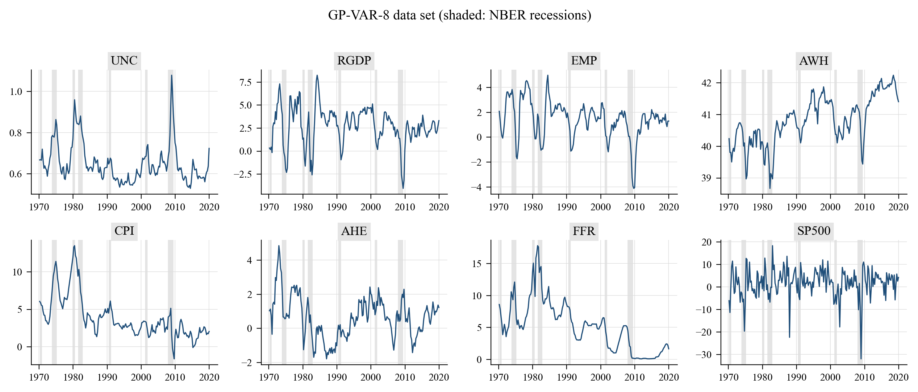
The model is estimated on standardised data with $p = 5$ lags, stochastic volatility, the semi-automatic $(\kappa,\xi)$ grid (20 × 50 points), 2 000 burn-in and 2 000 posterior draws; GIRFs use 100 evenly spaced posterior draws, all 195 histories and 5 simulated future paths per history. Uncertainty is ordered first (an uncertainty shock moves every variable on impact; the paper shows in Appendix C.2 that the ordering has a negligible effect on the GIRFs — gpvar.ordering_robustness reproduces that check).
5.2 In-sample features (Figures 5 and 6 of the paper)
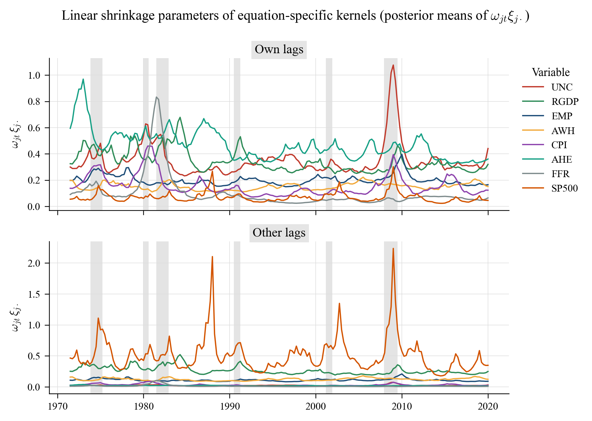
Posterior means of the "linear shrinkage" $\omega_{jt}\xi_{j\cdot}$ — the diagonal of the re-scaled kernels — for own and other lags (recessions shaded). As in the paper, less shrinkage is applied to own lags than to other lags and the amount of shrinkage rises sharply in recessions (early 1980s, 2008–09):
Posterior interquartile ranges of the inverse length scales $\kappa_{j1}$ (own lags, blue) and $\kappa_{j2}$ (other lags, green). Own-lag kernels are consistently "rougher" (larger $\kappa$) than other-lag kernels, whose effect is close to linear:
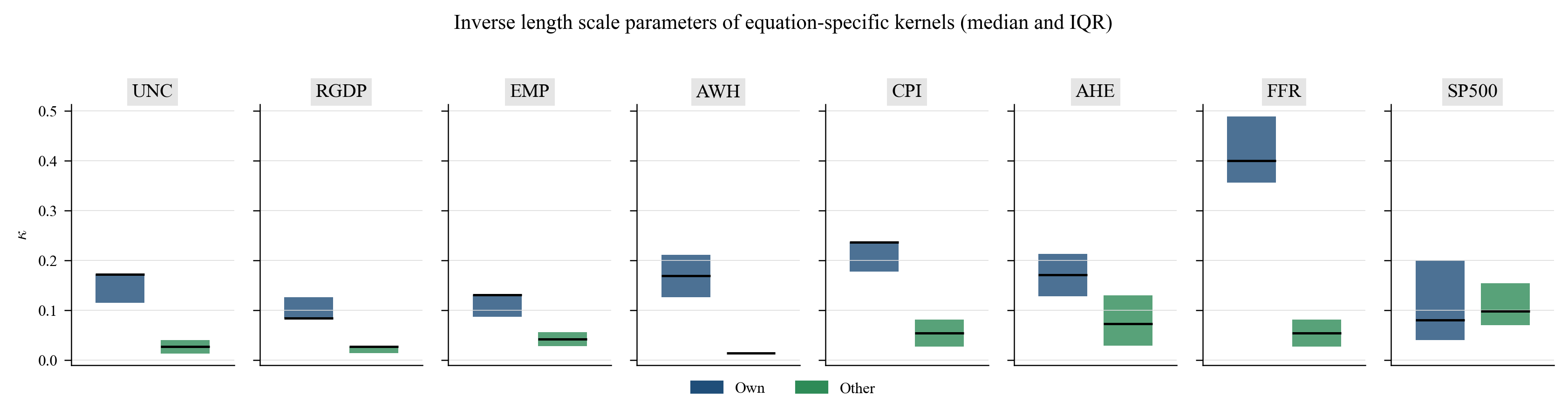
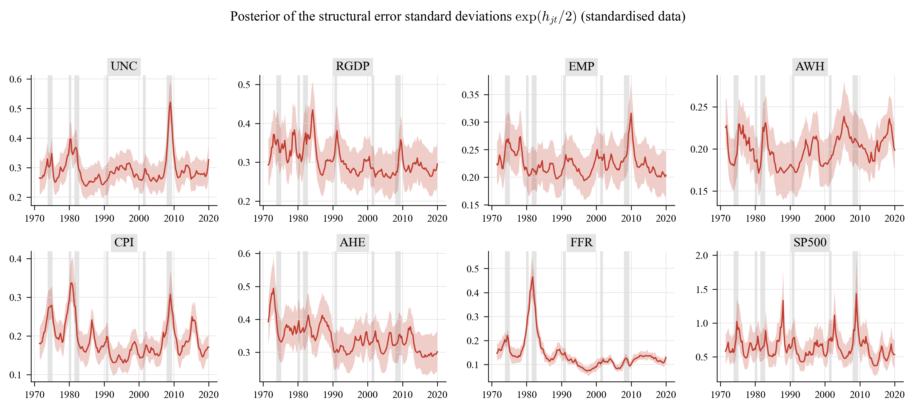
Posterior summaries of the kernel hyperparameters (median and interquartile range; $\xi$ on the paper's grid $[0.04, 4]$, $\kappa$ on $[0.1\bar\kappa, 2\bar\kappa]$) and of the stochastic-volatility state equations. Independence-MH acceptance rates for the log-volatility paths: UNC 0.72, RGDP 0.84, EMP 0.89, AWH 0.80, CPI 0.44, AHE 0.81, FFR 0.09, SP500 0.59 (the FFR equation is the hardest one because its conditional variance collapses at the zero lower bound, as the paper notes).
Kernel hyperparameters (outputs/tables/gpvar8_hyperparameters):
| Variable | kappa own | xi own | kappa other | xi other |
|---|---|---|---|---|
| UNC | 0.171 [0.114, 0.171] | 3.838 [3.677, 4.000] | 0.027 [0.013, 0.040] | 0.121 [0.040, 0.363] |
| RGDP | 0.084 [0.084, 0.126] | 3.515 [3.111, 3.838] | 0.027 [0.014, 0.027] | 2.788 [2.060, 3.434] |
| EMP | 0.130 [0.087, 0.130] | 3.758 [3.515, 3.919] | 0.042 [0.028, 0.056] | 2.060 [1.252, 2.869] |
| AWH | 0.169 [0.126, 0.211] | 3.758 [3.515, 3.919] | 0.014 [0.014, 0.014] | 3.030 [2.464, 3.515] |
| CPI | 0.237 [0.177, 0.237] | 3.919 [3.758, 4.000] | 0.054 [0.027, 0.081] | 0.525 [0.202, 1.010] |
| AHE | 0.170 [0.128, 0.213] | 3.758 [3.596, 3.919] | 0.072 [0.029, 0.130] | 0.040 [0.040, 0.202] |
| FFR | 0.400 [0.356, 0.489] | 3.919 [3.838, 4.000] | 0.054 [0.027, 0.081] | 0.282 [0.040, 0.767] |
| SP500 | 0.080 [0.040, 0.200] | 0.040 [0.040, 0.121] | 0.098 [0.070, 0.154] | 0.929 [0.525, 1.414] |
SV state-equation parameters (outputs/tables/gpvar8_sv_parameters):
| Variable | mu_h | rho_h | sigma^2_h | h_0 |
|---|---|---|---|---|
| UNC | -2.477 [-2.732, -2.230] | 0.789 [0.638, 0.887] | 0.067 [0.037, 0.123] | -2.614 [-3.311, -1.862] |
| RGDP | -2.396 [-2.673, -2.088] | 0.756 [0.564, 0.879] | 0.068 [0.032, 0.154] | -2.424 [-3.160, -1.732] |
| EMP | -2.997 [-3.315, -2.692] | 0.746 [0.557, 0.875] | 0.053 [0.031, 0.103] | -2.980 [-3.583, -2.369] |
| AWH | -3.232 [-3.501, -3.023] | 0.767 [0.559, 0.894] | 0.038 [0.023, 0.068] | -3.033 [-3.493, -2.494] |
| CPI | -3.361 [-3.795, -3.024] | 0.869 [0.771, 0.924] | 0.076 [0.038, 0.122] | -3.446 [-4.242, -2.677] |
| AHE | -2.157 [-2.467, -1.898] | 0.790 [0.590, 0.902] | 0.056 [0.032, 0.102] | -1.938 [-2.573, -1.341] |
| FFR | -4.055 [-4.551, -3.518] | 0.934 [0.889, 0.965] | 0.055 [0.036, 0.079] | -3.875 [-4.700, -3.087] |
| SP500 | -0.945 [-1.498, -0.493] | 0.705 [0.487, 0.841] | 0.304 [0.134, 0.779] | -0.989 [-2.381, 0.287] |
The contemporaneous coefficients of $Q$ (horseshoe prior) are in outputs/tables/gpvar8_Q.md: e.g. the impact effect of uncertainty on GDP growth, $q_{\mathrm{RGDP,UNC}}$, has posterior median $-0.20$ with $P(q>0)=0.004$.
5.3 Uncertainty shocks: GP-VAR-8 versus a linear BVAR (Figure 7)
Average generalized impulse responses (posterior median and 68 % bands, averaged over all 195 histories) to a positive one-standard-deviation uncertainty shock, compared with the recursive IRFs of a Minnesota BVAR-8 estimated on the same data:
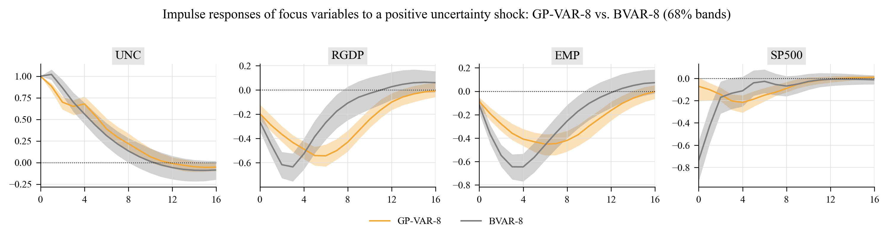
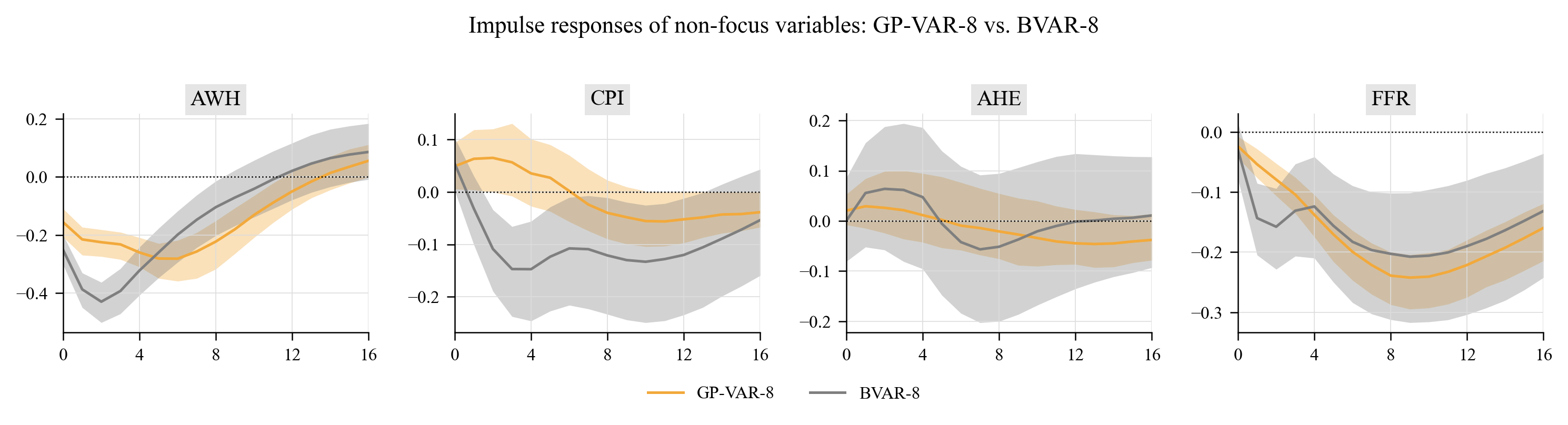
Both models agree on the qualitative picture (higher uncertainty lowers output growth, employment, hours, stock returns and the policy rate), but the GP-VAR responses of real activity peak later (five to six quarters after the shock versus three for the BVAR) and die out more slowly, and stock prices react on impact more mildly than in the linear model. Average GIRFs to a positive one-standard-deviation shock at selected horizons (posterior median and 68 % band, responses in standard-deviation units of the standardised data):
| Variable | h=0 | h=1 | h=4 | h=8 | h=12 | h=16 |
|---|---|---|---|---|---|---|
| UNC | 1.000 [1.000, 1.000] | 0.885 [0.826, 0.919] | 0.679 [0.571, 0.767] | 0.219 [0.139, 0.339] | -0.010 [-0.066, 0.061] | -0.053 [-0.098, -0.004] |
| RGDP | -0.195 [-0.246, -0.120] | -0.289 [-0.340, -0.208] | -0.487 [-0.568, -0.426] | -0.430 [-0.507, -0.335] | -0.100 [-0.165, -0.028] | -0.008 [-0.059, 0.058] |
| EMP | -0.087 [-0.146, -0.052] | -0.192 [-0.250, -0.139] | -0.408 [-0.466, -0.322] | -0.419 [-0.515, -0.338] | -0.163 [-0.250, -0.088] | -0.002 [-0.064, 0.053] |
| AWH | -0.156 [-0.207, -0.109] | -0.215 [-0.269, -0.173] | -0.260 [-0.309, -0.208] | -0.222 [-0.317, -0.151] | -0.050 [-0.111, 0.017] | 0.056 [-0.001, 0.111] |
| CPI | 0.049 [0.006, 0.094] | 0.063 [0.004, 0.119] | 0.035 [-0.027, 0.101] | -0.040 [-0.090, 0.022] | -0.052 [-0.097, -0.000] | -0.039 [-0.067, 0.000] |
| AHE | 0.021 [-0.008, 0.053] | 0.029 [-0.015, 0.084] | 0.012 [-0.042, 0.095] | -0.021 [-0.075, 0.055] | -0.045 [-0.087, 0.023] | -0.038 [-0.078, 0.014] |
| FFR | -0.024 [-0.043, -0.008] | -0.054 [-0.076, -0.028] | -0.138 [-0.175, -0.105] | -0.239 [-0.287, -0.200] | -0.221 [-0.275, -0.180] | -0.160 [-0.214, -0.119] |
| SP500 | -0.071 [-0.204, 0.008] | -0.101 [-0.200, -0.042] | -0.216 [-0.309, -0.152] | -0.090 [-0.124, -0.033] | -0.007 [-0.037, 0.019] | 0.009 [-0.010, 0.026] |
Notes: Responses in standard-deviation units of the (standardised) variables; horizons in quarters.
Peak responses (outputs/tables/gpvar8_girf_peaks) for the three shock configurations:
| shock | variable | impact | peak | peak_horizon | peak_q16 | peak_q84 | cumulative |
|---|---|---|---|---|---|---|---|
| positive 1 sd | UNC | 1.000 | 1.000 | 0 | 1.000 | 1.000 | 5.394 |
| positive 1 sd | RGDP | -0.195 | -0.543 | 6 | -0.631 | -0.450 | -4.740 |
| positive 1 sd | EMP | -0.087 | -0.451 | 6 | -0.547 | -0.368 | -4.323 |
| positive 1 sd | AWH | -0.156 | -0.281 | 6 | -0.358 | -0.218 | -2.488 |
| positive 1 sd | CPI | 0.049 | 0.065 | 2 | -0.000 | 0.120 | -0.150 |
| positive 1 sd | AHE | 0.021 | -0.046 | 13 | -0.093 | 0.018 | -0.249 |
| positive 1 sd | FFR | -0.024 | -0.242 | 9 | -0.295 | -0.204 | -2.903 |
| positive 1 sd | SP500 | -0.071 | -0.216 | 4 | -0.309 | -0.152 | -1.373 |
| negative 1 sd | UNC | -1.000 | -1.000 | 0 | -1.000 | -1.000 | -3.726 |
| negative 1 sd | RGDP | 0.195 | 0.341 | 5 | 0.291 | 0.387 | 3.078 |
| negative 1 sd | EMP | 0.087 | 0.261 | 3 | 0.208 | 0.311 | 2.551 |
| negative 1 sd | AWH | 0.156 | 0.201 | 1 | 0.159 | 0.251 | 1.724 |
| negative 1 sd | CPI | -0.049 | -0.062 | 1 | -0.115 | -0.005 | -0.286 |
| negative 1 sd | AHE | -0.021 | -0.028 | 1 | -0.078 | 0.015 | 0.148 |
| negative 1 sd | FFR | 0.024 | 0.148 | 9 | 0.120 | 0.183 | 1.886 |
| negative 1 sd | SP500 | 0.071 | 0.143 | 4 | 0.094 | 0.195 | 0.871 |
| positive 2 sd | UNC | 2.000 | 2.000 | 0 | 2.000 | 2.000 | 7.534 |
| positive 2 sd | RGDP | -0.390 | -0.847 | 5 | -0.968 | -0.714 | -6.345 |
| positive 2 sd | EMP | -0.174 | -0.709 | 5 | -0.827 | -0.593 | -6.129 |
| positive 2 sd | AWH | -0.311 | -0.440 | 5 | -0.557 | -0.337 | -3.474 |
| positive 2 sd | CPI | 0.098 | 0.112 | 1 | 0.007 | 0.214 | -0.531 |
| positive 2 sd | AHE | 0.041 | -0.064 | 12 | -0.129 | 0.032 | -0.308 |
| positive 2 sd | FFR | -0.048 | -0.357 | 8 | -0.413 | -0.298 | -4.287 |
| positive 2 sd | SP500 | -0.143 | -0.313 | 3 | -0.466 | -0.184 | -1.818 |
Notes: Peak = largest absolute posterior-median response; 68% credible interval at the peak horizon; cumulative = sum of median responses over 0-16 quarters.
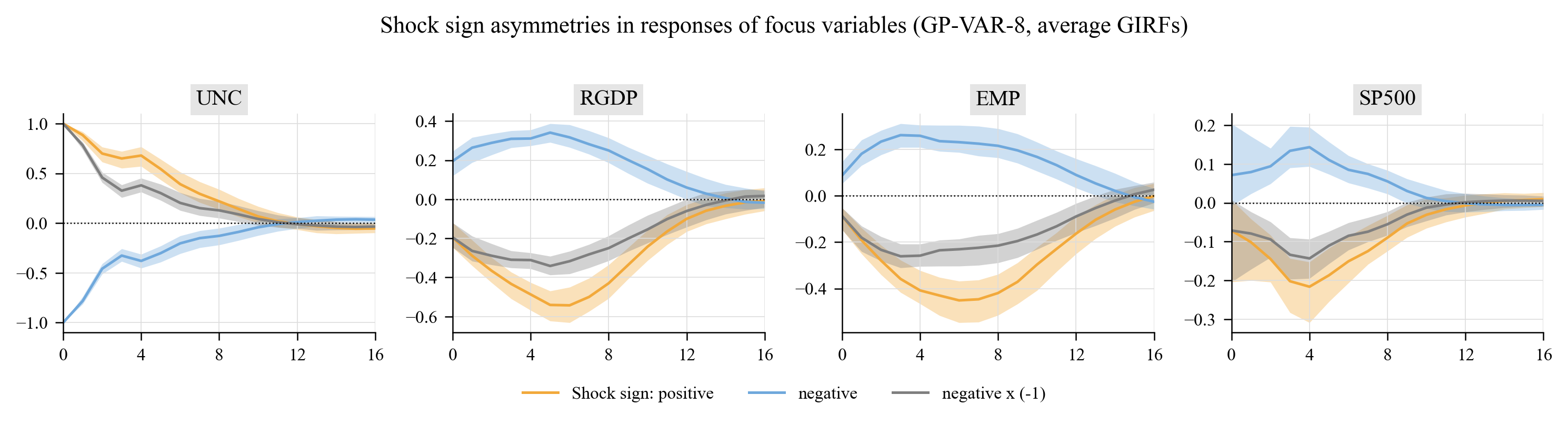
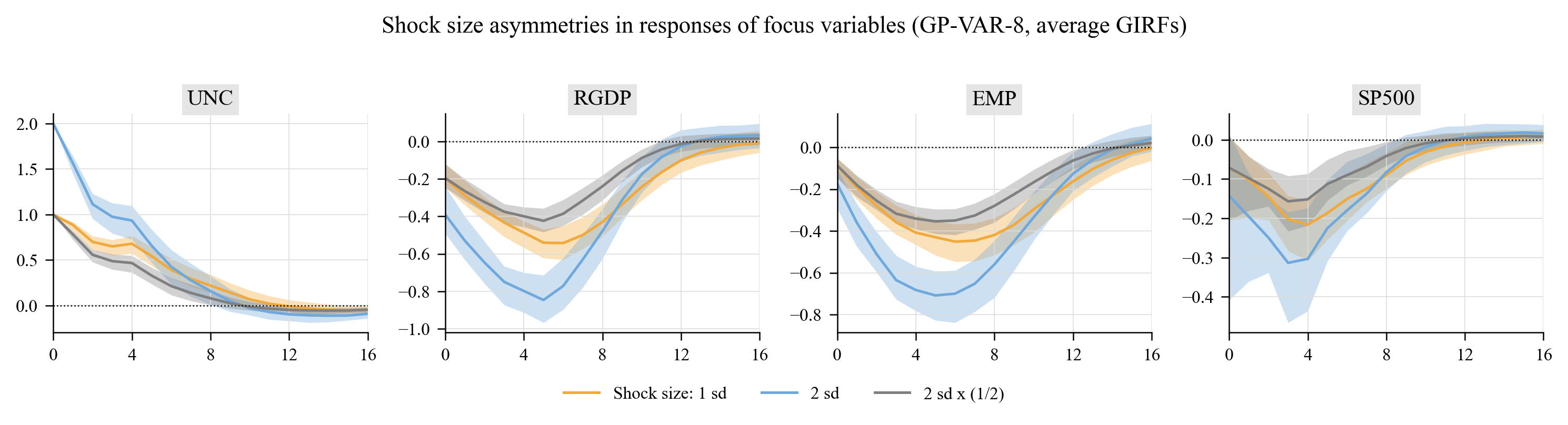
5.4 Sign and size asymmetries (Figures 9 and 10)
Responses to a positive (orange) and a negative (blue) shock, with the negative response mirrored (grey) so that a linear model would give identical orange and grey lines:
Responses to a one- and a two-standard-deviation shock, with the latter halved (grey) — proportionality would make orange and grey coincide:
The asymmetries are statistically sharp. Sign asymmetry: posterior median of $\delta^+_h + \delta^-_h$ (zero under linearity) with the posterior probability that it is positive:
| Variable | h=1 | h=4 | h=8 |
|---|---|---|---|
| UNC | 0.098 (1.00) | 0.291 (1.00) | 0.092 (0.93) |
| RGDP | -0.023 (0.00) | -0.170 (0.00) | -0.178 (0.00) |
| EMP | -0.010 (0.00) | -0.142 (0.00) | -0.197 (0.00) |
| AWH | -0.015 (0.00) | -0.100 (0.00) | -0.090 (0.00) |
| CPI | 0.001 (0.64) | -0.003 (0.46) | -0.043 (0.07) |
| AHE | 0.002 (0.77) | 0.009 (0.65) | -0.000 (0.49) |
| FFR | -0.003 (0.04) | -0.037 (0.00) | -0.094 (0.00) |
| SP500 | -0.022 (0.01) | -0.075 (0.01) | -0.030 (0.16) |
Notes: Under a linear model the responses to positive and negative shocks are mirror images and the statistic is zero.
Positive uncertainty shocks produce a larger endogenous uncertainty response and larger declines in GDP growth, employment, hours and stock returns than the mirror image of negative shocks, which is the paper's central result ("higher unexpected uncertainty has stronger effects on the economy than lower uncertainty"). Size asymmetry: ratio of the response to a 2-sd shock to the response to a 1-sd shock (2 under proportionality):
| Variable | h=1 | h=4 | h=8 |
|---|---|---|---|
| UNC | 1.76 | 1.38 | 0.72 |
| RGDP | 1.84 | 1.64 | 1.11 |
| EMP | 1.88 | 1.67 | 1.34 |
| AWH | 1.83 | 1.62 | 1.26 |
| CPI | 1.76 | 0.51 | 2.62 |
| AHE | 1.95 | 1.05 | 1.50 |
| FFR | 1.90 | 1.68 | 1.50 |
| SP500 | 1.93 | 1.40 | 0.92 |
Notes: Equal to 2 under proportionality (linear model).
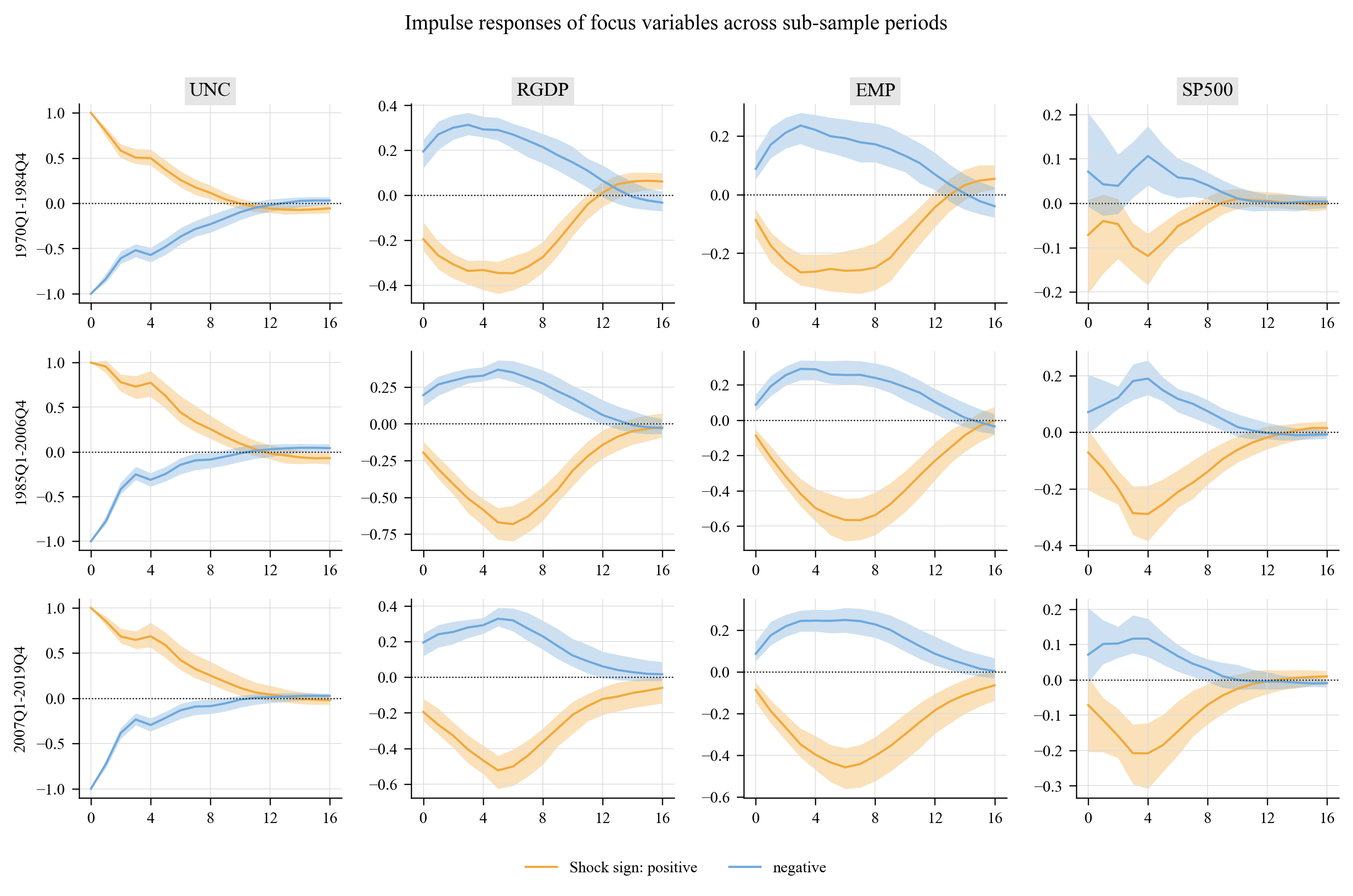
Large shocks have less-than-proportional effects on real activity (ratios of 1.6-1.7 at one year), exactly as in Figure 10 of the paper. Peak responses by sub-sample (outputs/tables/gpvar8_girf_peaks_by_period) show that the effects were weakest in the great-inflation period and strongest during the great moderation (peak GDP-growth response $-0.35$ vs $-0.68$ standard deviations), in line with the paper's Figure 11.
5.5 Asymmetries over time (Figures 11, 12 and C.6)
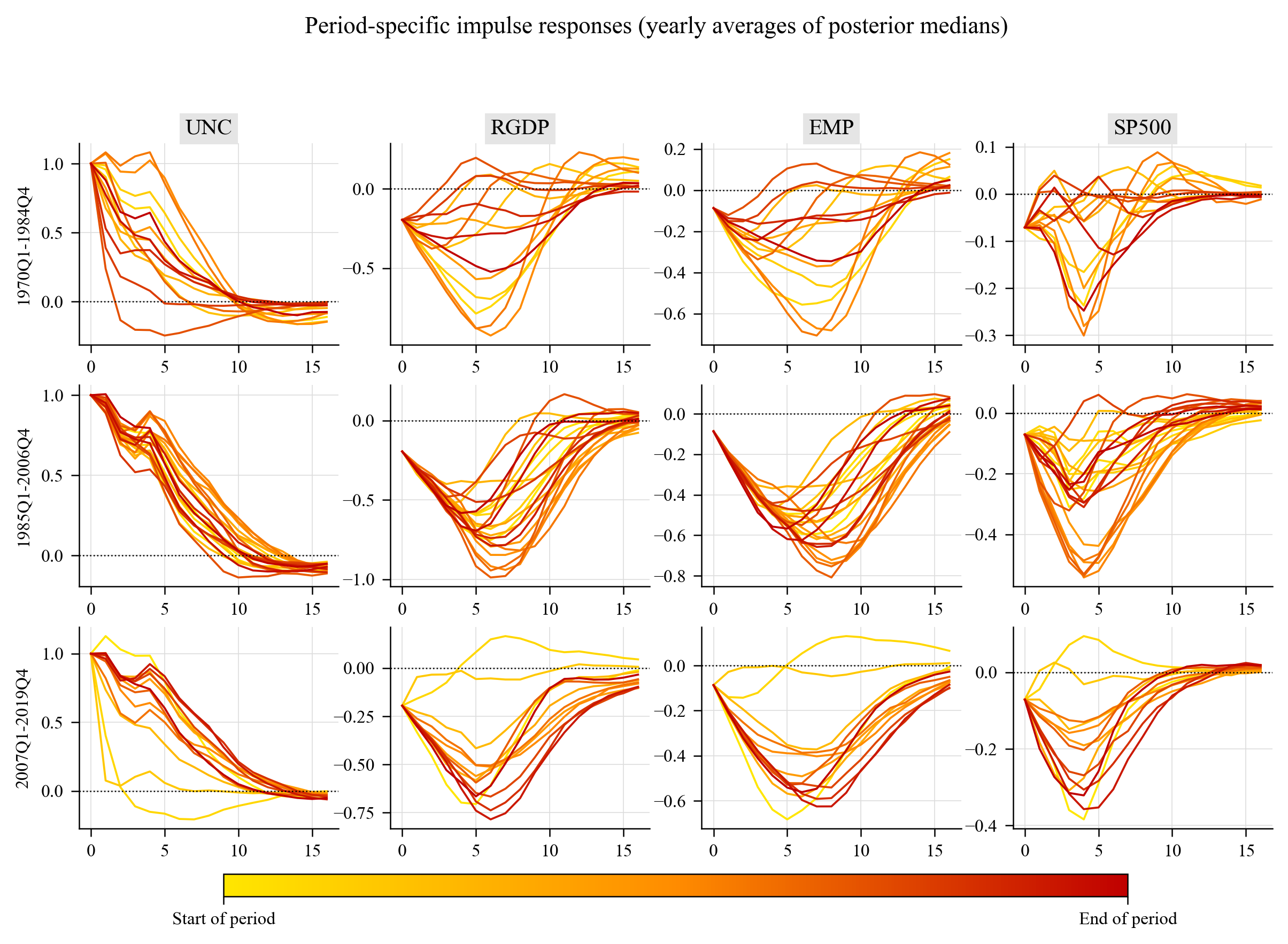
Sub-sample averages of the GIRFs (great inflation 1970Q1–1984Q4, great moderation 1985Q1–2006Q4, post-great-moderation 2007Q1–2019Q4):
Yearly averages of the posterior-median GIRFs within each sub-sample (yellow = start of the period, red = end):
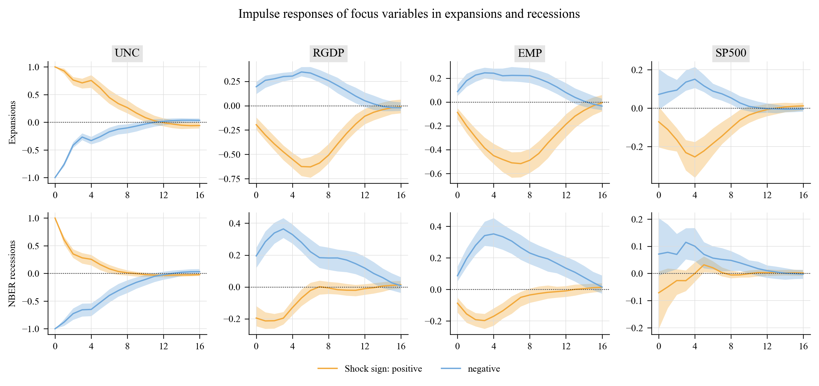
GIRFs conditional on the state of the business cycle (NBER expansions versus recessions):
5.6 Volatility, diagnostics and forecasts
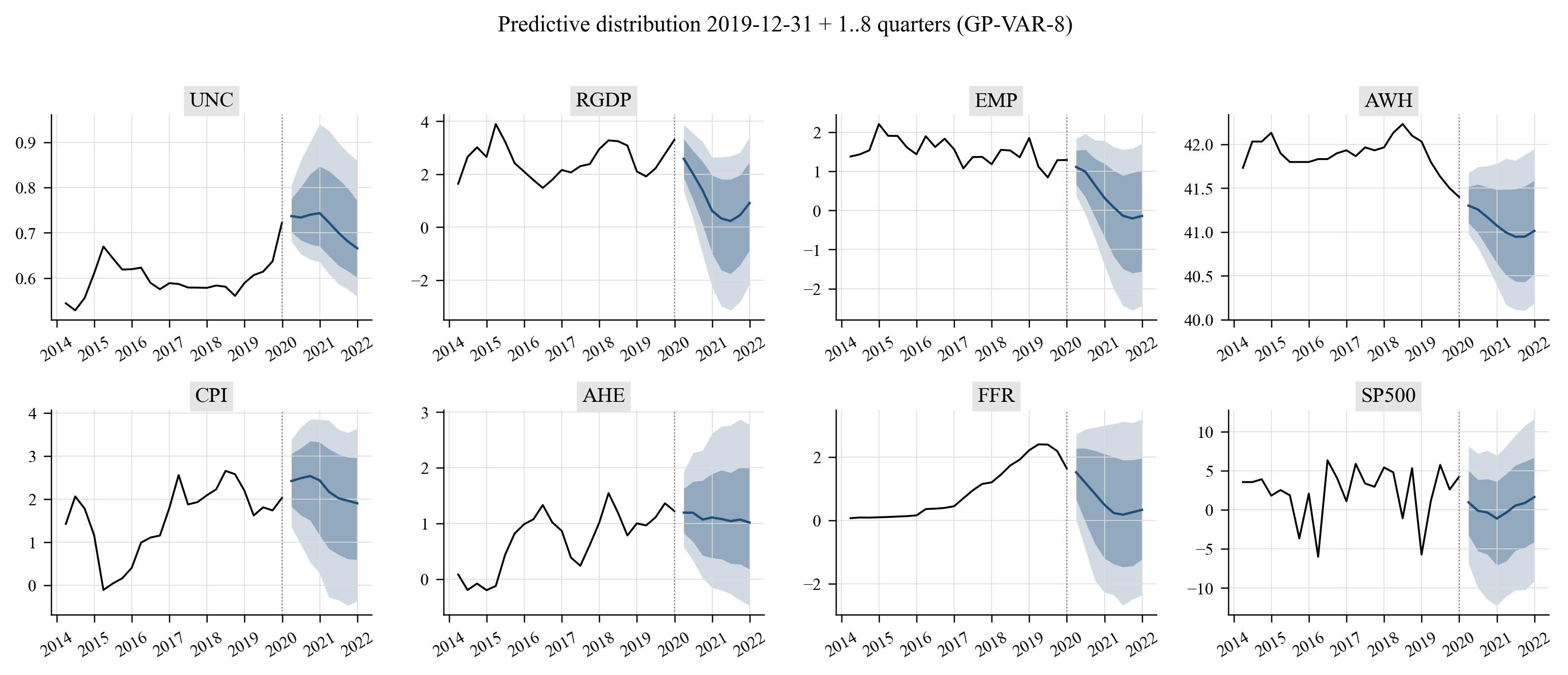
Predictive distribution eight quarters beyond the end of the sample (5/16/50/84/95 % quantiles):
MCMC traces of $\kappa$, $\xi$ and $\rho_h$ per equation are in outputs/figures/gpvar8_mcmc_traces.png; the non-focus-variable versions of every GIRF figure (figC4, figC5, figC7, figC9, figC10) and all tables are in outputs/.
6. Simulation study (Section 4 of the paper)
examples/02_simulation_study.py simulates the paper's three-equation DGP (linear equation with $t_3$ shocks, structural break at $t=100$, sine/quadratic non-linearities, random-walk SV, T = 200) and fits the GP-VAR. Posterior of $f_j$, $g_j$, $m_j = f_j+g_j$ and $y_j$ (red, 90 % bands) against the truth (black) — the analogue of the paper's Figure 3:
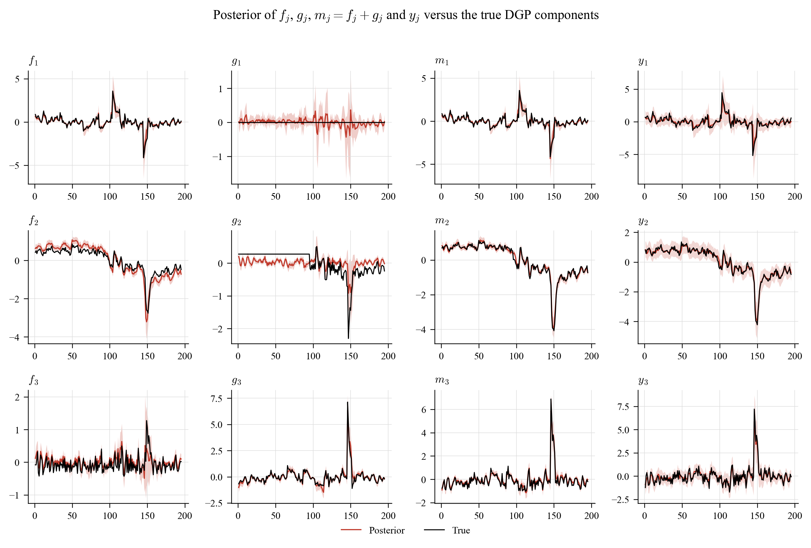
Correlation between the posterior median of $m_j$ and the true conditional mean over Monte Carlo replications of the DGP (the analogue of Table 1 of the paper, where the authors report 0.945, 0.929 and 0.754 over 100 replications):
| m1 | m2 | m3 | |
|---|---|---|---|
| Avg. | 0.987 | 0.965 | 0.925 |
| SD |
Notes: Results from 1 realisations of the Section 4 DGP with T = 200. Avg. is the average correlation, SD the standard deviation across realisations.
7. GP regression illustration (Section 2 of the paper)
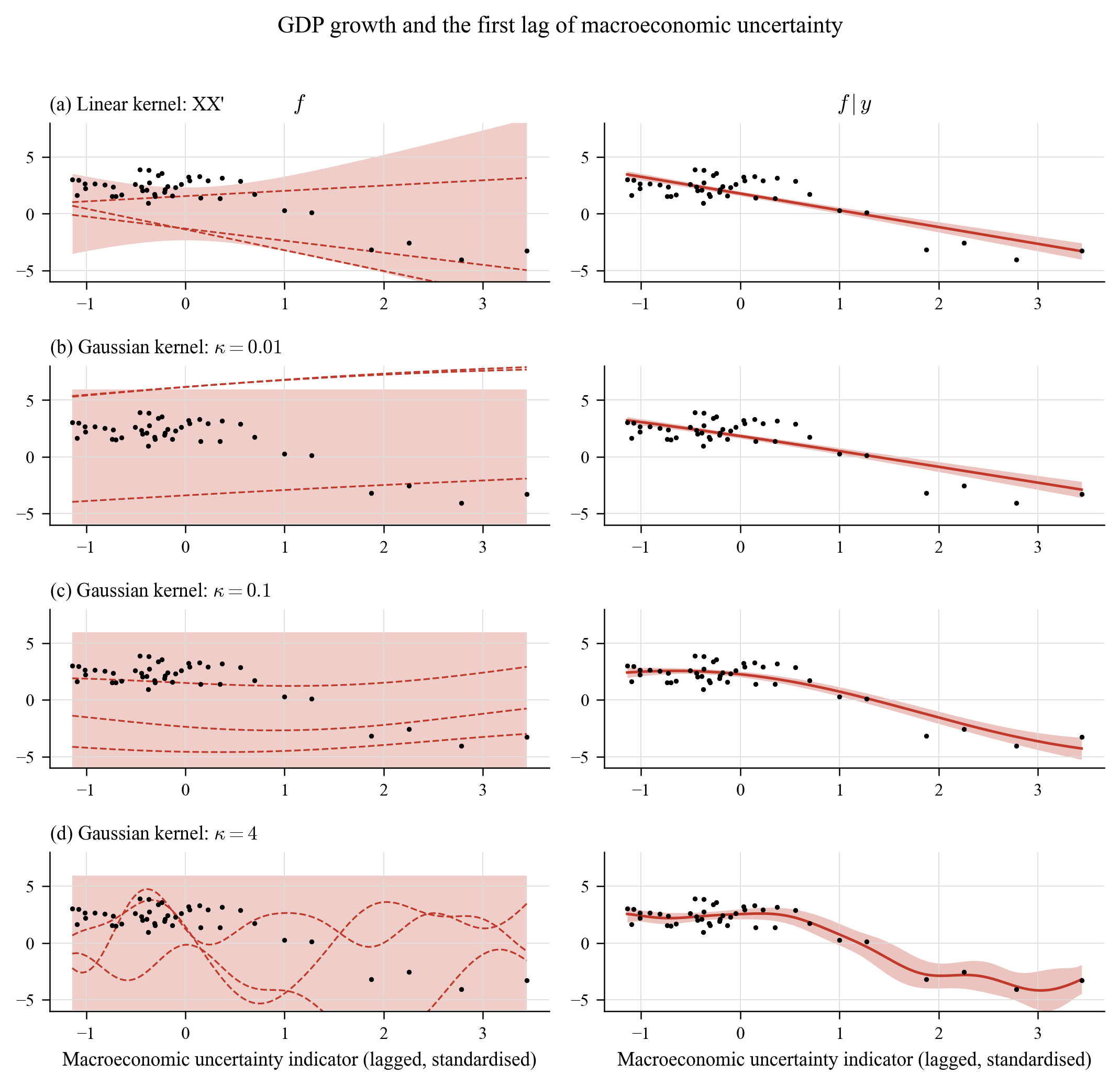
examples/01_gp_regression_illustration.py reproduces the univariate illustrations with the bundled data: US inflation on a linear trend (Figure 1), GDP growth on lagged macroeconomic uncertainty (Figure 2, below) and the persistence kernel of Appendix A.1. The role of $\kappa$ is exactly as described in the paper: $\kappa=0.01$ is essentially linear, $\kappa=0.1$ reveals the threshold at which high uncertainty starts to depress growth, $\kappa=4$ over-fits.
8. Forecast evaluation (Section 5.2 of the paper)
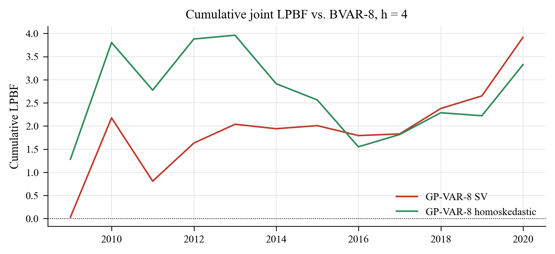
examples/04_forecast_evaluation.py runs the recursive (expanding-window) exercise for the GP-VAR-8 with SV, the homoskedastic GP-VAR-8 and a Minnesota BVAR-8, scoring one- and four-quarter-ahead density forecasts of RGDP, CPI and FFR with log predictive likelihoods (jointly and marginally) and CRPS. Log predictive Bayes factors relative to the BVAR (positive = better):
| variable | GP-VAR-8 SV (h=1) | GP-VAR-8 SV (h=4) | GP-VAR-8 homoskedastic (h=1) | GP-VAR-8 homoskedastic (h=4) | BVAR-8 (h=1) | BVAR-8 (h=4) | BVAR-8 (LPL) (h=1) | BVAR-8 (LPL) (h=4) |
|---|---|---|---|---|---|---|---|---|
| joint | -4.57 | 3.92 | -7.55 | 3.33 | 0.00 | 0.00 | -38.18 | -62.66 |
| RGDP | -0.73 | 2.74 | -0.42 | 4.12 | 0.00 | 0.00 | -14.51 | -24.63 |
| CPI | -2.18 | 2.67 | -4.26 | -0.01 | 0.00 | 0.00 | -10.96 | -20.01 |
| FFR | -1.22 | 1.76 | -2.13 | 0.73 | 0.00 | 0.00 | -12.96 | -23.74 |
Notes: Recursive design, origins 2007Q4 to 2018Q4 every 4 quarters; joint = RGDP, CPI and FFR. The last column block reports the benchmark's log predictive likelihoods.
Average CRPS by model, horizon and variable is in outputs/tables/table02b_crps.md.
With 12 annual origins (2007Q4–2018Q4, 400 + 400 MCMC draws per origin), the GP-VAR-8 with SV improves on the linear benchmark at the one-year horizon (joint LPBF +3.9; +2.7 for GDP growth, +2.7 for inflation, +1.8 for the funds rate) while the BVAR is better one quarter ahead, the same horizon pattern the paper reports in Table 2 (gains in predictive accuracy increase with the forecast horizon). The homoskedastic GP-VAR is close to the SV version at h = 4 but clearly worse at h = 1 for inflation and the funds rate, again as in the paper. Cumulative joint LPBFs over the evaluation sample:
9. Library reference
| Module | Purpose |
|---|---|
gpvar.GPVAR(Y, p, sv, hyper_scheme, n_kappa, n_xi, c_kappa, c_xi, hyper_sampling, restrict_g_mean, sv_priors, sv_hessian, sv_tries) |
Model specification and pre-computation (kernel eigendecompositions per equation and grid point). .fit(nburn, nsave, thin, seed) runs the MCMC and returns GPVARResults. |
gpvar.GPVARResults |
Posterior draws (f, g, h, Q, hyper, sv_params), summaries (hyper_summary, sv_summary, Q_summary, fitted, volatility, shrinkage_paths, fit_correlations), .predict(), .girf(), .save()/.load(). |
gpvar.girf(results, shock_var, size, sign, horizon, histories, n_sim, n_draws, shock_scale, sample_m) |
Generalized impulse responses for every history; returns GIRFResult with .summary(), .average(), .by_periods(), .yearly_medians(), .peak_table(), .state_dependence(), .mask_from_dates(). girf_sign_asymmetry, girf_size_asymmetry, ordering_robustness are convenience wrappers. |
gpvar.predict(results, horizon, n_sim, n_draws, sample_m) |
Simulation from the multi-step predictive distribution; ForecastResult.quantiles(). |
gpvar.log_predictive_score, gpvar.crps, gpvar.recursive_forecast_evaluation, gpvar.lpbf_table |
Density-forecast evaluation. |
gpvar.BVAR |
Natural-conjugate Minnesota BVAR benchmark with .predict() and Cholesky .irf(). |
gpvar.GPRegression |
Univariate GP regression (Gaussian / linear / persistence kernels) for the Section 2 illustrations. |
gpvar.simulate_paper_dgp, gpvar.simulate_replication_dgp |
Synthetic DGPs of the paper and of the replication archive. |
gpvar.data |
Bundled FRED-QD subset and JLN index, paper transformations (build_dataset, transform_series), NBER recessions, sub-sample definitions. |
gpvar.plots |
Journal-style figures: plot_girf, plot_girf_periods, plot_girf_time_variation, plot_shrinkage_paths, plot_kernel_boxplots, plot_volatility, plot_fit_components, plot_gp_illustration, plot_data, plot_forecast_fan, plot_lpl_cumulative, plot_trace. |
gpvar.tables |
Markdown / LaTeX (booktabs) / CSV writers and ready-made tables (hyper_table, sv_table, girf_horizon_table, girf_peak_table, asymmetry_table, size_asymmetry_table). |
gpvar.kernels, gpvar.sv, gpvar.priors, gpvar.predict |
Building blocks (kernel blocks with eigendecompositions, IMH volatility sampler, horseshoe, predictive engine). |
Key options of GPVAR:
hyper_scheme:"semi-automatic"(grid on both $\kappa$ and $\xi$, the paper's preferred specification),"semi-automatic-noscale"($\xi = 1$),"naive"($\kappa\in[0.1,2]$, $\xi=1$).hyper_sampling:"marginal"(default; samples $\vartheta$ with the latent function integrated out, then the function — a blocked step that mixes better) or"conditional"(the paper's Step 5/6 literally).sv: stochastic volatility (True) or homoskedastic errors (False, the "GP-VAR homoskedastic" of Table 2).sv_hessian:"dense"(exact Hessian for the IMH proposal, default) or"band"(the paper's tridiagonal approximation, cheaper for large $T$);sv_tries: accept/reject attempts per sweep from the same proposal.restrict_g_mean: grand-mean-zero restriction on $g_j$ (Appendix A.2).SVPriors(estimate_mu=False)removes the unconditional mean of the log-volatility process (eq. 3 of the paper literally).
10. How the implementation maps to the paper
| Paper | Implementation |
|---|---|
| Eq. (2) structural form with own/other lag functions | GPVAR (equation-by-equation), kernels.own_other_index |
| Eq. (3) SV process | sv.sample_sv_params (Beta(25,5) on $(\rho+1)/2$, IG(3, 0.2) on $\sigma^2_h$) |
| Eq. (4) SV-scaled GP priors, Gaussian kernel with scaling matrix $D$ | kernels.KernelBlock, posterior_draw |
| Section 3.3 median heuristic, grid $\kappa\in[0.1\bar\kappa,2\bar\kappa]$, $\xi\in[0.04,4]$, Gamma hyperpriors | kernels.median_heuristic, make_hyper_grid, log_gamma_prior |
| Section 3.4 conjugate posterior of $f_j$, pre-computed factors | eigendecomposition per $\kappa$ (all quantities $O(T^2)$ per draw) |
| Appendix A.2 sampling $g_j$ under $\iota'g_j=0$ (Cong, Chen, Zhou 2017) | GPVAR.fit, Steps 4 & 6 |
| Appendix A.3 log-volatilities: Newton–Raphson mode, band Hessian, independence MH | sv.sample_logvol_imh (band) / sv.sample_logvol_imh_dense |
| Appendix A.4 Steps 1–8 | GPVAR.fit |
| Section 3.5 / Appendix A.5 forecasts and GIRFs | predict.DrawContext, forecast.predict, girf.girf |
| Section 4 DGP, Table 1 | simulate.simulate_paper_dgp, GPVARResults.fit_correlations |
| Section 5.2 LPBFs | forecast.recursive_forecast_evaluation, lpbf_table |
| Figures 1–2, A.1 | GPRegression, plots.plot_gp_illustration |
| Figures 3, 5, 6, 7, 9, 10, 11, 12, C.4–C.10 | plots.* (see Section 4 above) |
Two deliberate differences from the paper are documented in docs/METHODOLOGY.md: the optional mean of the log-volatility process (on by default, as in the authors' R code) and the blocked ("marginal") hyperparameter step (the paper's conditional step is available with hyper_sampling="conditional"). The BVAR benchmark shipped here is homoskedastic (the paper's has SV).
11. Data
Two files ship in gpvar/datasets/ so that every example is reproducible offline:
fredqd_subset.csv— 26 series of FRED-QD (McCracken and Ng, 2020), vintage 2026-08, 1959Q1–2026Q2, with the FRED-QD transformation codes. Source: Federal Reserve Bank of St. Louis.jln_macro_uncertainty.csv— the JLN macroeconomic uncertainty index (h = 1, 3, 12), monthly 1960:07–2026:06 (August 2026 update), from Sydney C. Ludvigson's website.
gpvar.data.build_dataset(size=8 | 16, start, end) assembles the paper's GP-VAR-8 or GP-VAR-16 with the Table B.1 transformations (scheme="paper") or the FRED-QD codes (scheme="fred"); gpvar.data.fetch_fred_qd() downloads the latest full vintage. Samples extending through the pandemic (e.g. end="2025Q4") work out of the box (--end 2025Q4 in example 3 adds a 2020– sub-sample panel).
12. Performance and settings
Per MCMC sweep the cost is $O(M,T^2)$ for the GP draws plus one $T\times T$ Cholesky/inverse per equation for the volatility step; it does not grow with the number of lags or regressors. Measured on a laptop (pure NumPy, single process):
| Setting | Time |
|---|---|
| GP-VAR-8, T = 195, p = 5, 20 × 50 grid: pre-computation | ≈ 3 s |
| GP-VAR-8: one MCMC sweep (dense-Hessian SV step) | ≈ 0.13 s (4 000 sweeps ≈ 10 min) |
| GP-VAR-3 simulation (T = 195): one MCMC sweep | ≈ 0.04 s |
| GIRF, 195 histories × 5 future paths × 16 horizons, all 8 equations | ≈ 1 s per posterior draw (threads over draws); the three shock configurations of example 3 (100 draws each) take ≈ 4 min |
| Full example 3 (estimation + all GIRFs, figures and tables) | ≈ 15 min |
Memory: the eigendecompositions take $2M,n_\kappa T^2$ doubles (≈ 100 MB for M = 8, T = 195, $n_\kappa = 20$). For monthly data or M ≥ 32 reduce n_kappa, thin the GIRF draws (n_draws) and consider sv_hessian="band".
13. Repository layout
GP-VAR/
├── gpvar/                    the library
│   ├── model.py              GPVAR, GPVARResults (Gibbs sampler, Appendix A.4)
│   ├── kernels.py            Gaussian kernels, median heuristic, hyper grid, eigen-blocks
│   ├── sv.py                 independence-MH log-volatility sampler, SV parameters
│   ├── priors.py             horseshoe, SV priors
│   ├── predict.py            predictive engine shared by forecasts and GIRFs
│   ├── girf.py               generalized impulse responses and asymmetry analysis
│   ├── forecast.py           predictive simulation, LPL/LPBF/CRPS, recursive evaluation
│   ├── benchmarks.py         Minnesota BVAR benchmark
│   ├── simulate.py           Section 4 DGP and replication-archive DGP
│   ├── gp.py                 univariate GP regression (Section 2 illustrations)
│   ├── data.py               FRED-QD / JLN loaders, transformations, NBER dates
│   ├── plots.py, tables.py   journal-style figures and Markdown/LaTeX tables
│   └── datasets/             bundled data (see datasets/README.md)
├── examples/                 01 GP illustration · 02 simulation · 03 US uncertainty · 04 forecast evaluation · run_all.py
├── outputs/figures, outputs/tables   generated results (PDF/PNG, md/tex/csv)
├── tests/                    pytest suite
├── docs/METHODOLOGY.md       equation-by-equation mapping to the paper
├── docs/USER_GUIDE.md        syntax guide (same content as Section 4)
├── docs/CONCEPTS.md          the concepts behind the model, explained
├── docs/*.html, build_site.py  documentation site (GitHub Pages): https://merwanroudane.github.io/GP-VAR/
├── GPVAR_replication/        the authors' original R replication code (unchanged)
└── 2112.01995v3.pdf is not distributed; download the paper from arXiv
14. Citation, license, acknowledgements
If you use this code, please cite the original paper and this repository:
@article{hauzenberger2022gpvar,
  title   = {Gaussian Process Vector Autoregressions and Macroeconomic Uncertainty},
  author  = {Hauzenberger, Niko and Huber, Florian and Marcellino, Massimiliano and Petz, Nico},
  journal = {Journal of Business \& Economic Statistics (forthcoming); arXiv:2112.01995},
  year    = {2022}
}

@software{roudane2026gpvar,
  title   = {gpvar: Gaussian Process Vector Autoregressions with stochastic volatility in Python},
  author  = {Roudane, Merwan},
  year    = {2026},
  url     = {https://github.com/merwanroudane/GP-VAR}
}
Released under the MIT License. The FRED-QD data are provided by the Federal Reserve Bank of St. Louis; the uncertainty index by Jurado, Ludvigson and Ng (2015) — please cite them when using the data. The R code in GPVAR_replication/ is the authors' replication archive and remains their work.
Dr Merwan Roudane — merwanroudane920@gmail.com — https://github.com/merwanroudane
1 maintainer

Metadata
1 maintainer
Release files for gpvar 1.0.0
For a detailed explanation of source distributions (sdists) and built distributions (wheels), please see the package formats documentation.
Source distribution (sdist)
| File | Size | Uploaded | Provenance | |
|---|---|---|---|---|
| gpvar-1.0.0.tar.gz | 146.0 kB | Without provenance | Details |
Built distribution (wheel)
| File | Interpreter | ABI | Platform | Reset |
|---|---|---|---|---|
| gpvar-1.0.0-py3-none-any.whl | Python 3 | none | any | Details |
Total release size: 254.1 kB
Release files / gpvar-1.0.0.tar.gz
| Download URL | gpvar-1.0.0.tar.gz |
|---|---|
| Size | 146.0 kB |
| Tags | Source |
|
SHA-256 checksum How to use checksums |
af8279f75e13a229876cf517f571b5c18f32dcd9a38fbd5a848dc1ecde4638a5
|
|
BLAKE2b-256 checksum How to use checksums |
930967d0b1cac899bb69d1b605dc04346c5e60a6fbb9489bd7726c493d577a1a
|
| Upload date | |
|
Uploaded using Trusted Publishing? What is trusted publishing? |
No |
| Uploaded via |
twine/7.0.0 CPython/3.11.0
|
Release files / gpvar-1.0.0-py3-none-any.whl
| Download URL | gpvar-1.0.0-py3-none-any.whl |
|---|---|
| Size | 108.1 kB |
| Tags | Python 3 |
|
SHA-256 checksum How to use checksums |
65716722fd1ba8b95d5cda3e4bc4ae0c00f77ccf54bdf11f807f32861ce1d9e9
|
|
BLAKE2b-256 checksum How to use checksums |
3200d164dd10c79ae37258e6f941dc7e2345d35dcdef82980a5e2d13502c1409
|
| Upload date | |
|
Uploaded using Trusted Publishing? What is trusted publishing? |
No |
| Uploaded via |
twine/7.0.0 CPython/3.11.0
|
Security for gpvar 1.0.0
Provenance
Provenance describes where a file came from. On PyPI, provenance is shared via attestations, which provide a verifiable record of the build or publishing details. View details, limitations and caveats.
No provenance found
None of the files in this release were uploaded with provenance metadata.
A note on package security
PyPI is a repository for distributing packages, not a service for auditing them. While third-party security researchers and our staff do their best to detect and remove malicious packages, PyPI cannot guarantee the quality, security or suitability of any given package.
To learn more about protecting yourself from malicious actors, visit our package security documentation.













