Beautiful, animated, true-gradient Sankey diagrams — a Theme design system, overlays, dynamic colors and audio.

Project description
Animated Sankey Flow
A Python library for animated, gradient Sankey diagrams — the only one that renders true color gradients on the connections, with a full toolkit for storytelling videos: dark themes, dynamic colors, accounting‑style labels, a dynamic value axis, an optional time‑series overlay (bar‑chart‑race style), and background music straight from a local MP3 or a YouTube URL.


The Gradient Difference
No mainstream visualization library supports gradient colors on Sankey links. This one renders true color gradients that flow from the source node's color to the target node's color.
| Library | Sankey | Gradient links | Animation | Background music |
|---|---|---|---|---|
| Plotly | ✅ | ❌ solid only | ❌ | ❌ |
| Matplotlib | ❌ (no native) | – | – | – |
| Holoviews | ✅ | ❌ solid only | ❌ | ❌ |
| This library | ✅ | ✅ true gradients | ✅ | ✅ |
Each link is drawn as 50 color segments by default (configurable via n_segments) following a cubic‑Bézier curve.
Gallery
Every image below is rendered by the library — reproduce them all with the runnable gallery notebook.
Animate change over time — a decade of the energy transition, rendered to MP4 (shown here as a GIF):
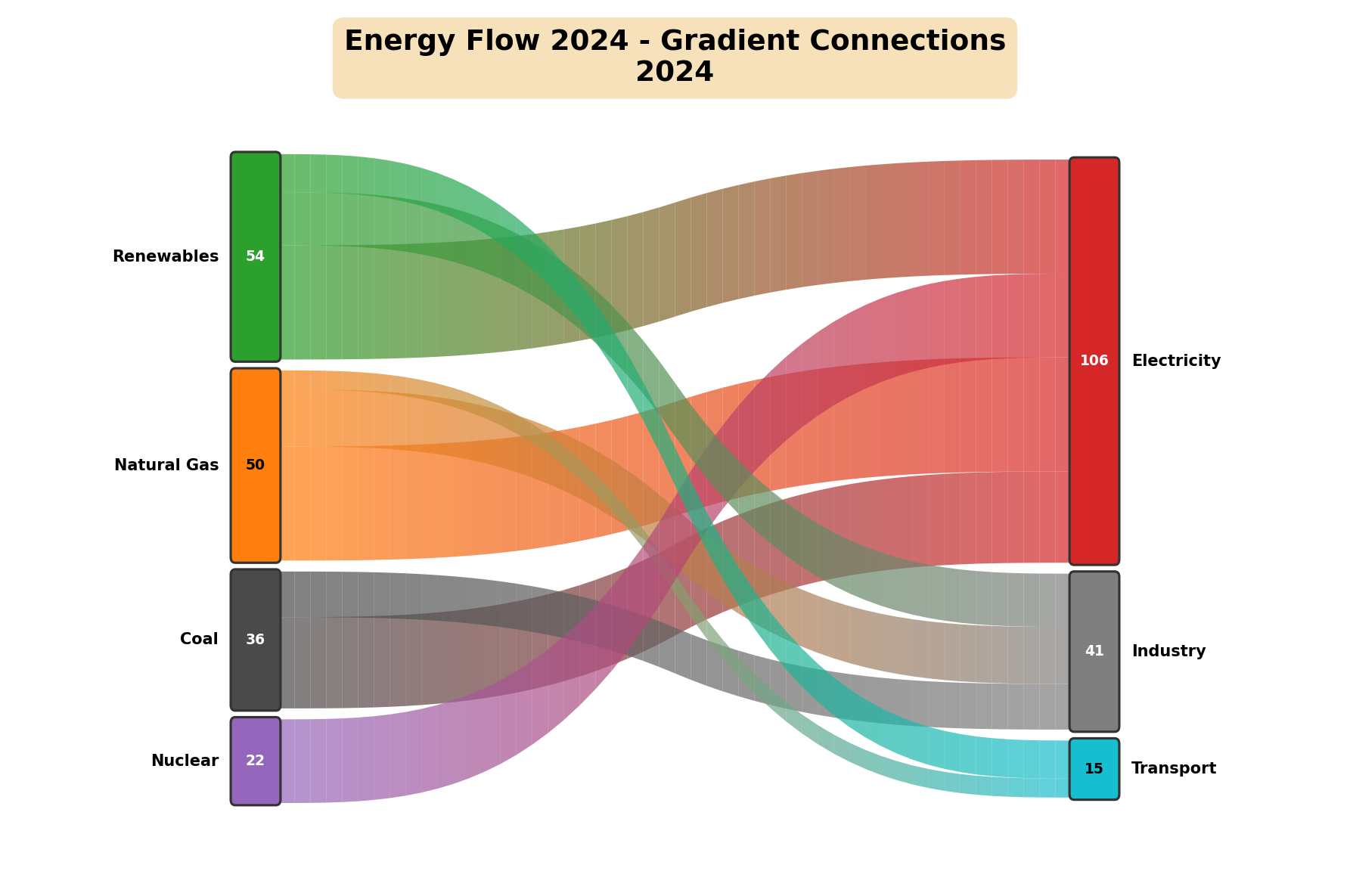
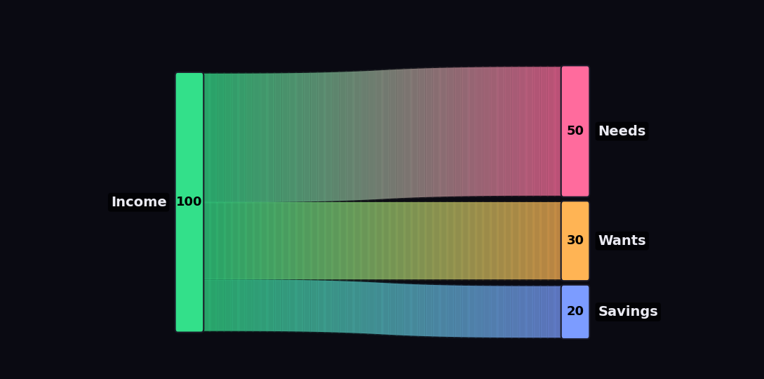
Any flow, beautifully — money, energy, users… width is volume and the color flows from source to target, so even a dense many‑to‑many diagram stays readable:
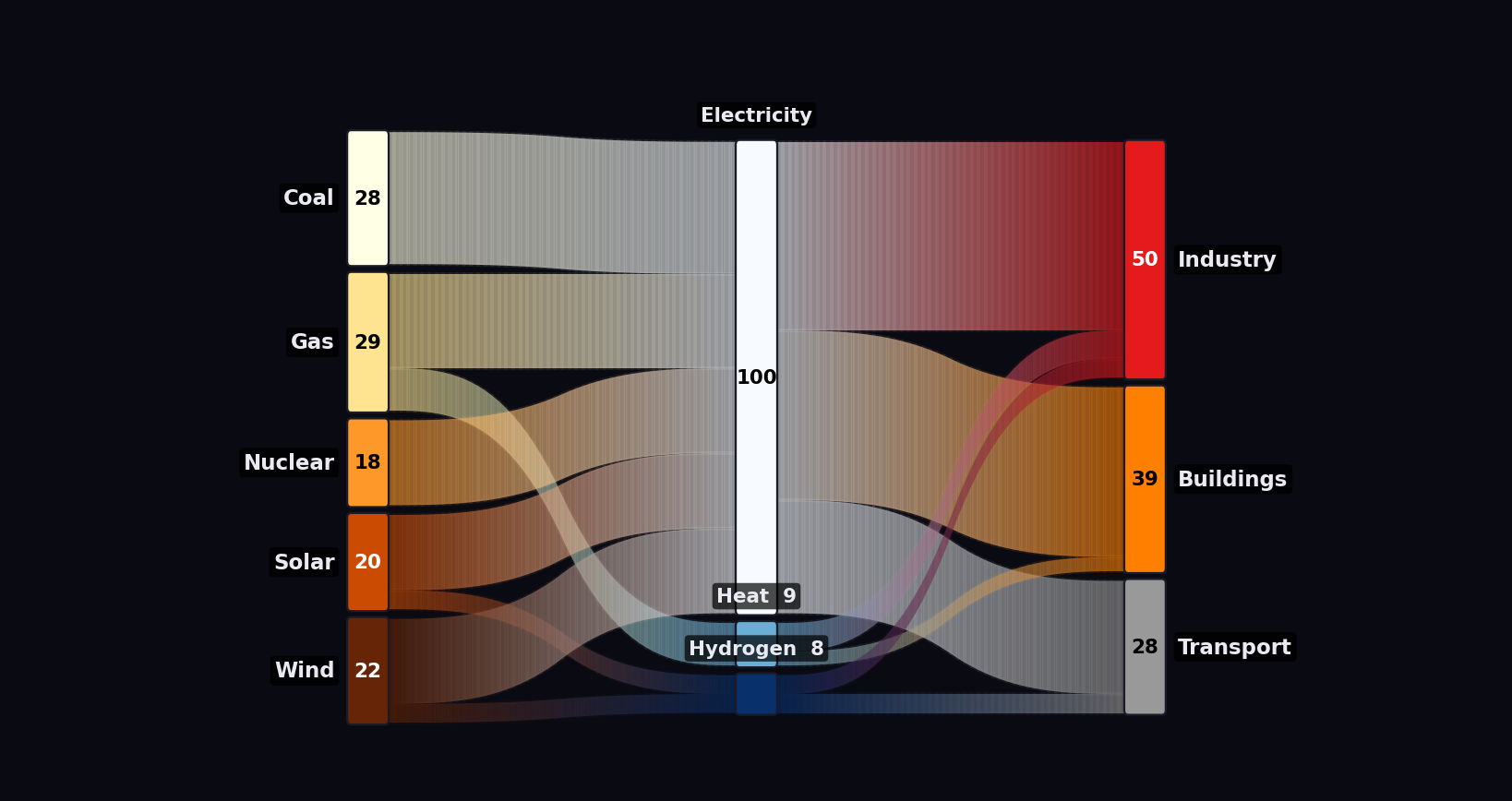
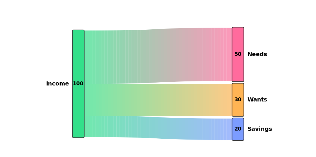
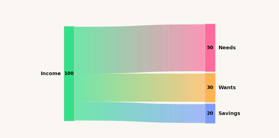
One look, three themes — the same data through the Theme design system: dark · light · editorial.
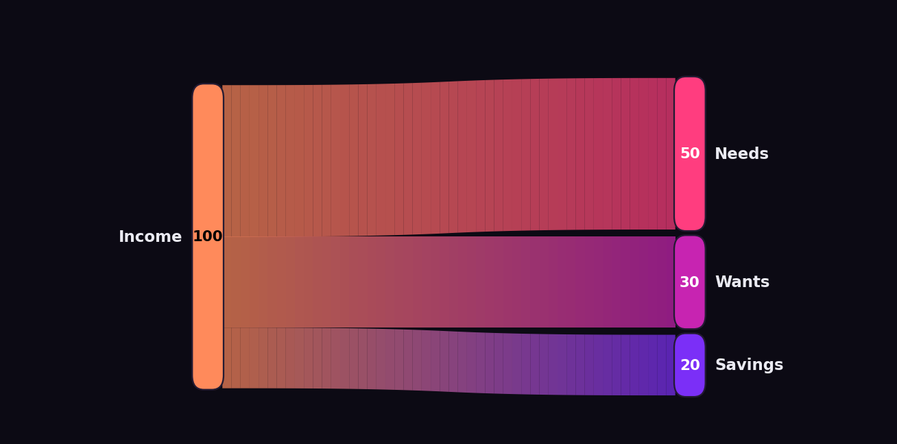
Make it yours — a custom Theme (pill‑shaped nodes, a heavier neon glow, a sunset palette):
What's new in this version
Everything below is additive and backward‑compatible — old code keeps working.
- 🎨
Themedesign system — one cohesive object for the whole look:Theme.dark(),Theme.light(),Theme.editorial(), or build your own (node.corner_radius,link.glow,type.base, …). See Themes. - 🌑 Dark theme + neon glow —
theme="dark",link_glow,link_alpha, custombg_color/label_color/node_edge_color/title_text_color. - 🎨 Dynamic node colors — including a new
"intensity"mode (keeps each node's hue, brightens with value). - 🔀 Automatic crossing reduction — links are stacked by the other end's vertical position, so flows don't tangle.
- 📐 Absolute scale —
absolute_scale=Truemakes bars grow in true magnitude across frames (the "explosion" effect). - 🏷️ Custom value labels & accounting parentheses —
node_value_labels/node_value_labels_per_frame(e.g. show losses as(5)); small bars print the value next to the node name so negatives are never hidden. - 📊 Dynamic value Y‑axis on any node —
yaxis_node=...draws an evolving$ruler next to a node. - 📈 Optional time‑series overlay (bar‑chart‑race style) —
overlay_series=...adds a growing mini‑chart + a discreet "big number" in the footer (e.g. a stock price). Optional — the flow can stay the main focus. - 🎵 Background music —
audio_path="song.mp3"oraudio_url="https://youtu.be/..."(downloads via yt‑dlp, timestamps ignored), withaudio_startandaudio_fade.
Jump to the feature guide or the full NVIDIA example.
Installation
pip install gradient-sankey

# With optional extras used by some examples:
pip install "gradient-sankey[finance,audio]"   # finance = requests + yfinance, audio = yt-dlp
FFmpeg is a system dependency (not pip-installable) required for video/audio export.
Or from source, for development:
git clone https://github.com/FG-SC/gradient-sankey.git
cd gradient-sankey
pip install -e ".[dev]"
Or just the core dependencies without installing the package:
pip install -r requirements.txt
Required: matplotlib, pandas, numpy.
FFmpeg (needed for any video/audio export — static PNGs work without it):
- Windows:
choco install ffmpegor download from https://ffmpeg.org/ - Linux:
sudo apt install ffmpeg - macOS:
brew install ffmpeg
Optional extras:
yfinance— stock/financial series for the time‑series overlay.yt-dlp— background music from a YouTube URL (pip install yt-dlp; also needs FFmpeg).
Using it in Jupyter / VS Code
A ModuleNotFoundError in a notebook after a successful terminal install almost
always means the notebook's kernel points to a different Python than the one
your terminal pip used. Install into the running kernel instead — the %pip
magic does exactly that:
%pip install gradient-sankey
import gradient_sankey as gs; print(gs.__version__)
(Or pick the matching interpreter via the kernel selector.) Then explore the runnable gallery notebook.
Quick Start
Static gradient Sankey
import pandas as pd
from gradient_sankey import SankeyRaceMultiLayerParallel

df = pd.DataFrame([
    {"year": 2024, "source": "Coal",        "target": "Electricity", "value": 24},
    {"year": 2024, "source": "Natural Gas", "target": "Electricity", "value": 30},
    {"year": 2024, "source": "Renewables",  "target": "Electricity", "value": 30},
    {"year": 2024, "source": "Renewables",  "target": "Industry",    "value": 14},
])

layers = [["Coal", "Natural Gas", "Renewables"], ["Electricity", "Industry"]]

sankey = SankeyRaceMultiLayerParallel.from_dataframe(
    df=df, layers=layers,
    time_col="year", source_col="source", target_col="target", value_col="value",
)
sankey.save_frame("energy.png", title="Energy Flow 2024", figsize=(12, 8), dpi=150)
Animated video
Add more time periods and call animate():
sankey.animate(
    output_path="energy.mp4",
    title="Energy Transition",
    fps=24, duration_seconds=10.0,
    ranking_mode=True, stacked_mode=True,
)
Node names must be unique across all layers. If the same entity appears twice, suffix it:
"China (export)"vs"China (import)".
Core API
SankeyRaceMultiLayerParallel.from_dataframe(...)
| Param | Type | Default | Description |
|---|---|---|---|
df |
DataFrame | — | Flow data: time, source, target, value columns. |
layers |
List[List[str]] | — | Node layers, left → right. Each inner list is one column. |
time_col / source_col / target_col / value_col |
str | — | Column names. |
layer_palettes |
List | None | Optional per‑layer palette for auto‑coloring. |
node_colors |
Dict[str,str] | None | Explicit hex color per node (recommended). |
save_frame(...) — static image (PNG/PDF/SVG)
Key params: output_path, frame_index, title, figsize, dpi, ranking_mode, stacked_mode, n_segments, plus all the theme params (theme, bg_color, link_glow, …) and node_value_labels described below.
animate(...) — video (parallel render → FFmpeg)
The big one. Parameters grouped by purpose:
Output & timing — output_path, title, figsize, fps, duration_seconds, quality ("low"/"medium"/"high"), n_workers.
Layout — node_width, padding, font_size, bar_height_ratio, margin_top, margin_bottom, title_fontsize, n_segments.
Positioning — ranking_mode, stacked_mode, ascending, absolute_scale.
Theme — theme, bg_color, label_color, node_edge_color, title_text_color, title_bg_color, title_bg_alpha, link_alpha, link_glow.
Dynamic colors — dynamic_color_mode, dynamic_colormap.
Labels — node_value_labels_per_frame.
Value axis — yaxis_node, yaxis_suffix.
Time‑series overlay — overlay_series, overlay_label, overlay_color, overlay_value_suffix, overlay_x_labels, overlay_badge (corner tag, e.g. a ticker like "NVDA").
Audio — audio_path, audio_url, audio_start, audio_fade.
Each is explained with examples in the guide below.
Feature guide
1. Animation modes — ranking_mode × stacked_mode
ranking_mode |
stacked_mode |
Behavior | Use it for |
|---|---|---|---|
| ✅ | ✅ | Reorder by value and resize (default) | size + ranking changes |
| ✅ | ❌ | Reorder by value, uniform heights | pure ranking races |
| ❌ | ✅ | Fixed order, heights vary by value | tracking each node over time |
| ❌ | ❌ | Fixed order, uniform heights (only links animate) | stable comparisons |
sankey.animate(ranking_mode=False, stacked_mode=True) # e.g. an income statement (fixed order)

2. Absolute vs per‑frame scale — absolute_scale
By default (absolute_scale=False) each frame is normalized to fill the canvas — great for showing composition changes (margins, mix), and every frame stays readable.
Set absolute_scale=True to use a single global scale so bars grow in true magnitude across frames — the "watch it explode" effect (e.g. revenue going $1B → $82B literally gets taller).
sankey.animate(stacked_mode=True, ranking_mode=False, absolute_scale=True)
Tip: absolute scale is dramatic but back‑loaded if the series explodes late. Per‑frame fill + the dynamic Y‑axis or labels is often more legible.
3. Themes — the design system
Animation is the core, but a chart also has to be beautiful. How it looks is
controlled by one cohesive object, Theme, so you can dial in the design once
and reuse it. Three presets ship out of the box:
from gradient_sankey import Theme

sankey.animate("reel.mp4", theme=Theme.dark())        # near‑black bg, light labels
sankey.save_frame("frame.png", theme=Theme.light())   # classic white (default)
sankey.save_frame("print.png", theme=Theme.editorial())  # warm paper, charcoal ink
A Theme bundles a palette‑independent look: background, text color, and three
nested styles you can tweak field by field —
look = Theme.dark()
look.node.corner_radius   = 0.18   # pill‑shaped nodes
look.node.edge_color      = "#1a1a28"
look.node.label_plate_alpha = 0.0  # turn off the label backing plate
look.link.glow            = 3      # neon halo layers behind links (0 = off)
look.link.alpha           = 0.75   # link translucency
look.type.base            = 14     # typographic scale
sankey.animate("reel.mp4", theme=look)
| Group | Fields |
|---|---|
Theme |
background, text, title_text, title_bg, title_bg_alpha |
Theme.node (NodeStyle) |
width, corner_radius, pad, edge_color, edge_width, label_plate_alpha |
Theme.link (LinkStyle) |
alpha, glow, segments |
Theme.type (TypeScale) |
base, title |
Backward compatible: theme="dark"/"light" strings still work, and every
old styling keyword (bg_color, label_color, node_edge_color, link_glow,
font_size, …) still works as an override on top of the chosen theme:
sankey.animate(theme="dark", link_glow=1, bg_color="#0a0a12") # still valid
4. Dynamic node colors — dynamic_color_mode
Recolor nodes every frame based on their value/rank:
| Mode | Meaning |
|---|---|
"static" |
Fixed colors (default) |
"ranking" |
Color by rank within the layer (1st → last) |
"value" |
Color by value, normalized within each layer |
"global_value" |
Color by value, normalized across all frames |
"percentile" |
Color by percentile within the layer |
"intensity" |
Keeps each node's base hue, scales brightness by value (globally) — nodes "light up" as they grow |
sankey.animate(dynamic_color_mode="ranking",
               dynamic_colormap=["#FF1E56", "#FFC400", "#7CFF6B"])  # neon red→green
dynamic_colormap accepts a ColorPalette, any matplotlib colormap name, or a list of hex colors.
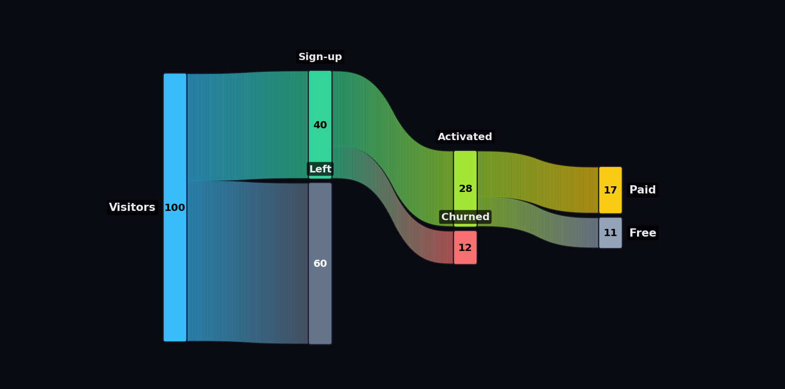
5. Uniform flows — color by position
For a clean, uniform look, give the i‑th node of every layer the same color (so each "track" of the flow is one consistent hue, and the gradient only appears where tracks split):
POS = ["#33E08A", "#FF2E97"]   # position 0 (kept) = green, position 1 (leak) = magenta
node_colors = {n: POS[i] for layer in layers for i, n in enumerate(layer)}
6. Negative values & accounting parentheses
Sankey links can't be negative, so values are sized by magnitude (abs). To keep sign information, pass custom label strings — negatives in (parentheses), accounting‑style:
def fmt(v):                       # 4.78 -> "4.8" ; -4.78 -> "(4.8)"
    s = f"{abs(v):.1f}" if abs(v) < 10 else f"{abs(v):.0f}"
    return f"({s})" if v < 0 else s

# static frame:
sankey.save_frame(..., node_value_labels={"Net Income": fmt(58), "Tax & Other": fmt(-4.78)})

# animation: one dict per data frame (aligned to the sorted time values)
sankey.animate(..., node_value_labels_per_frame=[{node: fmt(v) for node, v in frame.items()} for frame in frames])
When a bar is too small to fit text inside, the value is automatically printed next to the node's name — so negatives like Tax+Other (4.8) are always visible.
7. Dynamic value Y‑axis on a node
Attach a subtle, evolving $ ruler to one node (typically the first/biggest). Its tick labels grow over time, making the magnitude readable even when bars are per‑frame normalized:
sankey.animate(
    yaxis_node="Revenue",   # node to attach the axis to
    yaxis_suffix="B",       # tick labels become "$0", "$25B", "$50B", ...
)
Ticks use "nice" round steps and rescale automatically; the node's name moves to the top of its bar to make room.
8. Time‑series overlay (optional, bar‑chart‑race style)
Optional. If you only want the flow, skip this entirely. When present, it adds a growing mini‑chart + a discreet "big number" in a reserved footer band.
Pass one value per data frame (aligned to the sorted time values). The chart is drawn bar‑chart‑race style: the curve always fills the width, the time (X) axis evolves (window start→now remapped to full width), the Y axis is a running max, and the "now" point sits at the right edge.
sankey.animate(
    overlay_series=stock_close_per_quarter,        # e.g. NVDA adjusted close, one per frame
    overlay_label="NVDA stock  ($, split-adj.)",
    overlay_color="#7CFF6B",
    overlay_value_suffix="",                       # "" for price, "B" for billions, ...
    overlay_x_labels=quarter_labels,               # e.g. ["2015 Q2", ...] → year ticks on the X axis
    margin_bottom=0.20,                            # reserve the footer so it doesn't collide with the flow
)
The overlay is horizontally aligned with the Sankey (first node → last node).
9. Background music — local MP3 or YouTube URL
Mux a soundtrack into the exported MP4. Two ways:
A) Local MP3
sankey.animate(
    audio_path="song.mp3",
    audio_start=41.5,   # seconds into the track to begin (e.g. start at the drop)
    audio_fade=1.5,     # fade in/out seconds
)
B) Straight from a YouTube URL (requires yt-dlp + FFmpeg)
Just pass the URL — timestamps in the link are ignored, the full track is fetched and extracted to MP3 automatically:
sankey.animate(
    audio_url="https://www.youtube.com/watch?v=WITxo7OfMVM&t=90s",  # &t=90s is ignored
    audio_start=269,   # start the song at 4:29 in the video
)
The audio is faded in/out and trimmed to the video length. You can also download a track yourself:
from gradient_sankey import youtube_to_mp3
path = youtube_to_mp3("https://youtu.be/WITxo7OfMVM", out_dir="music")
⚠️ Rights: downloaded tracks may be copyrighted. For Instagram Reels, the in‑app licensed music library is the safe path; muxed audio is handy for platforms without one (e.g. LinkedIn) but may be flagged by Content‑ID. Use tracks you have the rights to.
Full example: NVIDIA income‑statement reel
examples/render_nvidia_reel.py combines almost every feature: real SEC EDGAR data, a fixed‑order P&L waterfall, dynamic $ Y‑axis, accounting parentheses for loss quarters, a bar‑chart‑race stock overlay, dark/neon theme, and background music.
# Local MP3, full 90s reel from 2009:
python examples/render_nvidia_reel.py --start-year 2009 --duration 90 \
    --audio "examples/music/song.mp3" --audio-start 269

# Or pull the music from YouTube (timestamp ignored):
python examples/render_nvidia_reel.py --start-year 2015 --duration 45 \
    --audio-url "https://www.youtube.com/watch?v=WITxo7OfMVM" --audio-start 269
| Flag | Default | Description |
|---|---|---|
--start-year |
2015 | First year of the series |
--duration |
45 | Video length (seconds) |
--audio |
— | Local MP3 path |
--audio-url |
— | YouTube URL (needs yt‑dlp) |
--audio-start |
0 | Seconds into the track to begin |
examples/nvidia_dre.py is the data layer: it scrapes 4 clean series from the SEC EDGAR XBRL API (Revenue, Gross Profit, Operating Income, Net Income) and derives the "leak" flows as residuals (COGS = Revenue − Gross, etc.) so the Sankey always balances.
Color palettes
Three ways to specify colors, all interpolated continuously:
from gradient_sankey import ColorPalette, get_palette_colors

get_palette_colors(ColorPalette.VIRIDIS, n_colors=5)        # built-in enum
get_palette_colors("RdYlGn", n_colors=10)                   # any matplotlib colormap
get_palette_colors(["#FF0000", "#FFFF00", "#00FF00"], 8)    # custom hex list (interpolated)
get_palette_colors(ColorPalette.OCEAN, 8, reverse=True)     # reversed
Built‑in palettes: RAINBOW, VIRIDIS, PLASMA, INFERNO, PASTEL, DARK, EARTH, OCEAN, SUNSET, NEON.
How gradients work
Each link is split into n_segments quads along a cubic‑Bézier S‑curve. Segment color is a linear RGB interpolation from source to target: color = source + t·(target − source), t ∈ [0,1].
n_segments |
Quality | Speed |
|---|---|---|
| 10–20 | visible bands | fast |
| 50 (default) | smooth | balanced |
| 100+ | ultra‑smooth | slower |
Performance
Parallel rendering scales with cores:
| Config | 240 frames |
|---|---|
| Serial | ~70s |
| Parallel (4 workers) | ~32s (2.2×) |
Tips: lower quality or fps while iterating; raise them only for the final render. High quality (dpi 200) × many frames is the main cost.
Project structure
gradient-sankey/
├── gradient_sankey.py        # the library (all features, single module)
├── pyproject.toml            # packaging (core deps + [finance]/[audio] extras)
├── requirements.txt          # core deps only
├── examples/
│   ├── gallery.py            # feature cookbook (inputs, palettes, modes, dynamic colors)
│   ├── nvidia_dre.py         # SEC EDGAR scraper -> P&L flows (cached to nvidia_dre_wide.csv)
│   ├── nvidia_dre.csv        # committed flows (reproducible/offline fallback)
│   ├── render_nvidia_reel.py # full reel (CLI: --start-year/--duration/--audio[-url]/--refresh)
│   ├── render_nvidia_poc.py  # single static frame
│   ├── us_energy_flow.py     # conservative-flow example (+ shipped demo .mp4)
│   └── company_financials.py # non-conservative (P&L) example
├── tests/                    # pytest suite (run `pytest`; render tests need ffmpeg)
├── assets/                   # gifs / images for docs
├── README.md  ·  CHANGELOG.md  ·  LICENSE
Troubleshooting
- FFmpeg not found — install it (see Installation); required for any video/audio.
- YouTube audio fails —
pip install yt-dlp; ensure FFmpeg is on PATH. If a video won't download, installingdenoresolves yt‑dlp's JS‑runtime warning. - Nodes in wrong positions — node names must be unique across layers.
- Negative values look odd — bars are sized by magnitude; use
node_value_labels(_per_frame)to show(parentheses). - Growth not visible — use
absolute_scale=True, ayaxis_node, and/or anoverlay_series. - Memory errors on large animations — reduce
figsize/dpi/frames, or lowern_workers. - Windows multiprocessing — guard your script with
if __name__ == "__main__": mp.freeze_support().
License
MIT — see LICENSE.
Release history Release notifications | RSS feed


Download files
Download the file for your platform. If you're not sure which to choose, learn more about installing packages.
Source Distribution
Built Distribution
Filter files by name, interpreter, ABI, and platform.
If you're not sure about the file name format, learn more about wheel file names.
Copy a direct link to the current filters
File details
Details for the file gradient_sankey-1.2.1.tar.gz.
File metadata
- Download URL: gradient_sankey-1.2.1.tar.gz
- Upload date:
- Size: 2.2 MB
- Tags: Source
- Uploaded using Trusted Publishing? No
- Uploaded via: twine/6.2.0 CPython/3.14.0
File hashes
| Algorithm | Hash digest | |
|---|---|---|
| SHA256 |
579b5bf2dcaa566435f9db6cbf4d046914c486c7373964ca1112d6810b391d6d
|
|
| MD5 |
4ede53d2ee1064bb944802d2cea07a9a
|
|
| BLAKE2b-256 |
2298b3779be1e8c561bf9ee08d5341eff8d5b323fa35527a18e634d13a175388
|
File details
Details for the file gradient_sankey-1.2.1-py3-none-any.whl.
File metadata
- Download URL: gradient_sankey-1.2.1-py3-none-any.whl
- Upload date:
- Size: 34.3 kB
- Tags: Python 3
- Uploaded using Trusted Publishing? No
- Uploaded via: twine/6.2.0 CPython/3.14.0
File hashes
| Algorithm | Hash digest | |
|---|---|---|
| SHA256 |
0cad19f8b07462fd69912963c5ec5489a04580380671a505372c22f7653f608c
|
|
| MD5 |
022dbe93a70b8c932fd1462c0422097b
|
|
| BLAKE2b-256 |
1a19b6c01fa51bb81efd242be3e7bab153af2f8110d48ed0fb3cc032bec5f2ca
|


