
Graphene Tools
A set of tools to generate the interaction of helium with uniaxially strained graphene (in the armchair direction) using optimized Lennard-Jones parameters from Nichols et al. and to print command line parameters for use with quantum Monte Carlo (QMC) software located at code.delmaestro.org. Code to generate figures for 1D and 2D potential interactions included as well. Please cite the origial paper as:
@article{Nichols2016,
  title = {Adsorption by design: Tuning atom-graphene van der Waals interactions via mechanical strain},
  author = {Nichols, Nathan S. and Del Maestro, Adrian and Wexler, Carlos and Kotov, Valeri N.},
  journal = {Phys. Rev. B},
  volume = {93},
  issue = {20},
  pages = {205412},
  numpages = {14},
  year = {2016},
  month = {May},
  publisher = {American Physical Society},
  doi = {10.1103/PhysRevB.93.205412},
  url = {https://link.aps.org/doi/10.1103/PhysRevB.93.205412}
}
Installation
You can install Graphene Tools from PyPI:
pip install graphenetools-py
How to use
Some command line tools have been included for convenience. Avaiable options are dermined by:
python -m graphenetools
For example, to run the listed command to print the parameters corresponding to a roughtly square box commensurate with the $C_{1/3}$ phase with strain $\delta=0.25$ and 100 adsorption sites use:
python -m gt_rs 5 --strain 0.25
or
gt_rs 5 --strain 0.25
Advanced usage
Better usage of the Graphene Tools package can be achieved by importing the pacakge directly into your project or notebook environment using from graphenetools import gt. Some advanced usage cases are discussed below.
Lattice vectors
Generate basis, lattice, and reciprocal lattice vectors for uniaxially strained graphene.
strain = 0.50 # Strain value in armchair direction
Am, An, b1, b2, gm, gn = gt.get_graphene_vectors(strain)
$C_{1/3}$ phase lattice vectors can be generated too!
strain = 0.50 # Strain value in armchair direction
Am_c_one_third, An_c_one_third = gt.get_graphene_c_one_third_vectors(strain)
Plot lattice
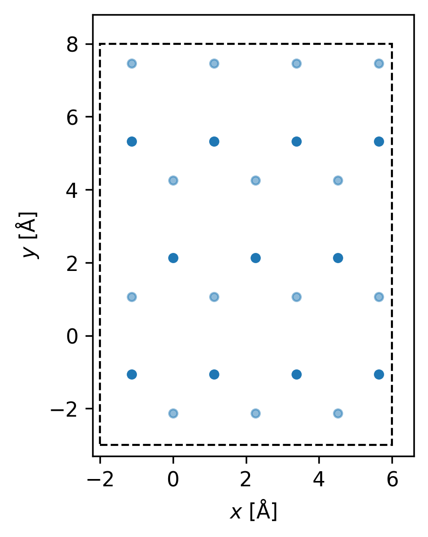
Plots of the graphene lattice can be made using the plot_graphene_lattice() function.
# Here we plot a funky box
box_dims = [-2.0,6.0,-3.0,8.0]
strain = 0.50
fig, ax = gt.plot_graphene_lattice(strain,box_dims)
fig.set_dpi(300)
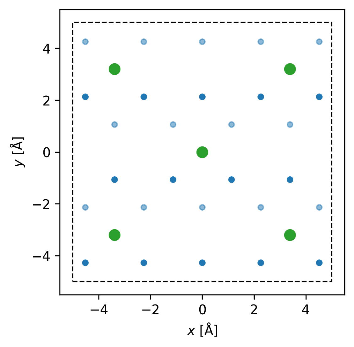
Additionally, the $C_{1/3}$ phase locations can be plotted along with the graphene lattice using the plot_graphene_lattice_with_c_one_third() function.
# If given a single float or int box dims is [-box_dims/2,box_dims/2,-box_dims/2,box_dims/2]
# Here we plot the graphene lattice and C1/3 adsorption sites
box_dims = 10
strain = 0.50
fig, ax = gt.plot_graphene_lattice_with_c_one_third(strain,box_dims)
fig.set_dpi(300)
Generate QMC parameters
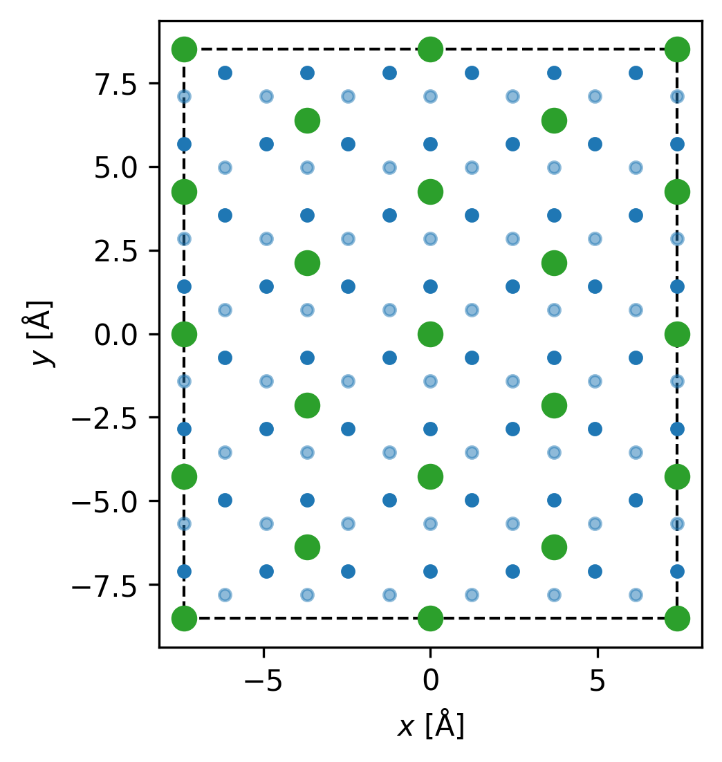
Simulation parameters to produce a roughly square simulation cell commensurate with the $C_{1/3}$ phase for use with QMC software hosted at code.delmaestro.org can be generated using the roughly_square() function and a plot of simulation cell generated using the roughly_square_plot() function.
# Here we plot roughly square plots commensurate with the C1/3 adsorption sites and print out the relevant PIMC parameters
strain = 0.00
n=2 # `(2n)^2` C1/3 adsorption sites
fig, ax = gt.roughly_square_plot(n,strain)
gt.roughly_square(n,strain) #print out the relevant PIMC parameters
fig.set_dpi(300)
-N 16 --Lx 14.757072880486835 --Ly 17.04
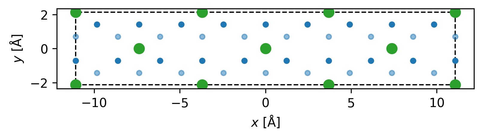
For non-"roughly square" command line parameters and plots use functions c_one_third_commensurate_command() and c_one_third_commensurate_command_plot().
# Here we plot a mostly rectangular plot commensurate with the C1/3 adsorption sites and print out the relevant PIMC parameters
strain = 0.00
m=3
n=1
fig, ax = gt.c_one_third_commensurate_command_plot(m,n,strain)
gt.c_one_third_commensurate_command(m,n,strain) #print out the relevant PIMC parameters
fig.set_dpi(300)
-N 6 --Lx 22.135609320730254 --Ly 4.26
Generate potential plots
The potential can also be calculated for the helium-graphene interaction using Graphene Tools. Here are some demonstrations at various strains.
0D potential plot (a single point)
The potential can be generate at a single point using the V_64() function. Optimized parameters to the Lennard-Jones potential are obtained using the get_LJ_parameters() function.
# Get optimized Lennard-Jones parameters for certain strain
strain = 0.00
conventional=True # Setting conventional to true will return the conventional parameters
sigma, epsilon = gt.get_LJ_parameters(strain,conventional=conventional)
_x = 0.00
_y = 0.00
_z = 3.00

# Generate helium-graphene interaction potential for a single point
carbon_carbon_distance=1.42
poisson_ratio=0.165
k_max=10000
potential="V" # can also generate the gradient or Laplacian by setting this variable to gradVx, gradVy, gradVz, or grad2V
gt.V_64(strain, sigma, epsilon, _x, _y, _z, carbon_carbon_distance=carbon_carbon_distance, poisson_ratio=poisson_ratio, k_max=k_max,potential=potential)
-158.92622261112095
1D potential plot
Here a 1D potential for a helium atom located above the graphene sheet is generated using the generate_V1D(). Note that the graphene sheets are centered on the center of the hexgonal unit (not centered on a carbon atom).
# Generate a 1D potential along z-direction at specific (x,y) location
strain = 0.00
x = 0.0
y = 0.0
z = gt.np.linspace(2.0,15.0,1001)
V = gt.generate_V1D(x,y,z,strain=strain) #Using default arguments (check function for extensive list)
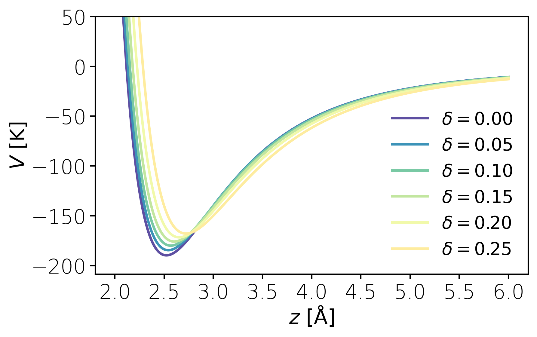
Plots for multiple values of strain can be generated using the plot_V1D() function.
x = 0.00
y = 0.00
z = gt.np.linspace(2,6,1001)
dpi = 300
strains = gt.np.linspace(0,.25,6)
mplstylefile = "./include/notebook.mplstyle"
fig, ax, V_array = gt.plot_V1D(x,y,z,strains=strains,mplstylefile=mplstylefile,dpi=dpi)
fig.savefig("V1D_optimized_close.png",bbox_inches="tight")
Minimum of 1D potential
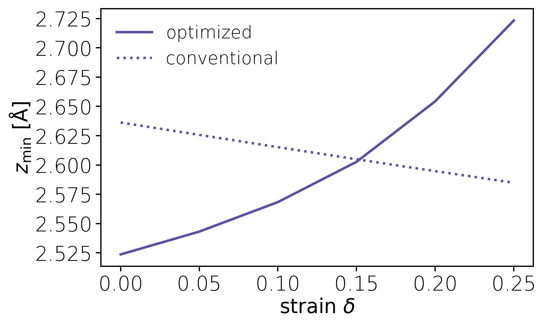
The minimum location and value of the potential for the different strain values can be determined using the get_z_min() and get_z_mins() functions.
# Get minimum potential and location above graphene sheet for a single strain value
strain = 0.00
z_min, V_min = gt.get_z_min(strain)

# Get minimum potential and location above graphene sheet for multiple strains
strains = gt.np.linspace(0,.25,6)

z_mins, V_mins = gt.get_z_mins(strains)
z_mins_conventional, V_mins_conventional = gt.get_z_mins(strains,conventional=True)
Note the different behavior when using the optmized parameters from [Nichols et al.] compared with using the conventional parameters.
#Plot z
mplstylefile = 'default'
with gt.plt.style.context(mplstylefile):
    fig, ax = gt.plt.subplots(dpi=300)
    ax.plot(strains,z_mins,label="optimized")
    ax.set_prop_cycle(None)
    ax.plot(strains,z_mins_conventional,linestyle=":",label=r"conventional")
    ax.set_xlabel(r"$\mathrm{strain}\ \delta$")
    ax.set_ylabel(r"$z_\mathrm{min}\ \mathrm{[\AA]}$")
    ax.legend()
    fig.savefig("zmin.png")
2D potential plot
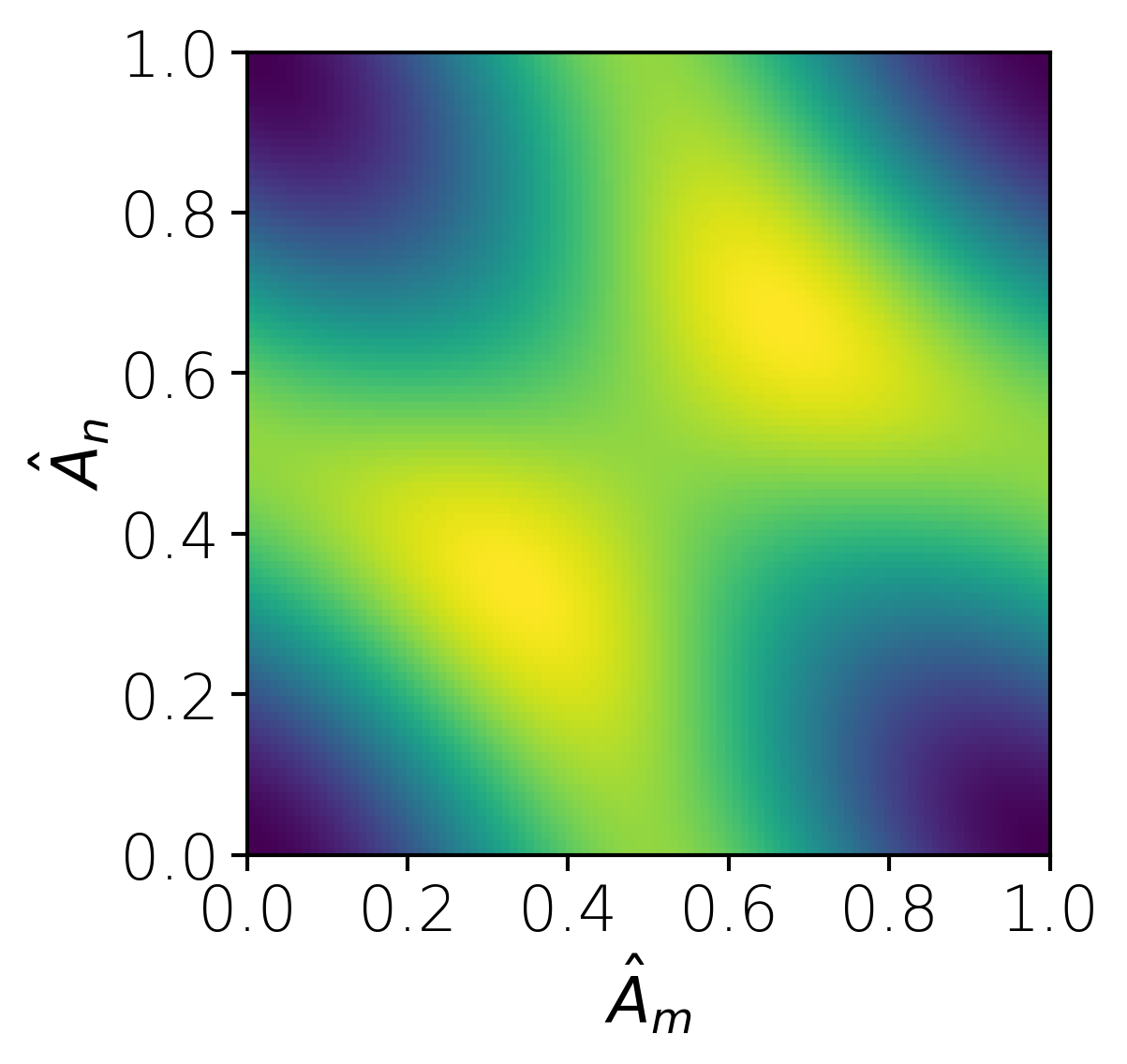
Here a 2D potential lookup table for a helium atom located above the graphene sheet is generated over the unit cell using the generate_V2D_uc().
strain = 0.00
resolution = 101
fn_prefix="./helium-graphene-2D-unit-cell"
z_min, V_min = gt.get_z_min(strain)

# Generate 2D lookup table on the unit cell for
data = gt.generate_V2D_uc(z_min, strain=strain, resolution=resolution, fn_prefix="./helium-graphene-2D-unit-cell")
Here is a visualization of the 2D lookup table.
fn = "helium-graphene-2D-unit-cell-conventional_V_strain_0.00000_z_2.63624_res_101.npz"
data = gt.np.load(fn)
mplstylefile = 'default'
with gt.plt.style.context(mplstylefile):
    fig,ax = gt.plt.subplots(dpi=300)
    ax.imshow(data["potential"].T,origin="lower",extent=[0,1,0,1])
    ax.set_xlabel(r"$\hat{A}_m$")
    ax.set_ylabel(r"$\hat{A}_n$")
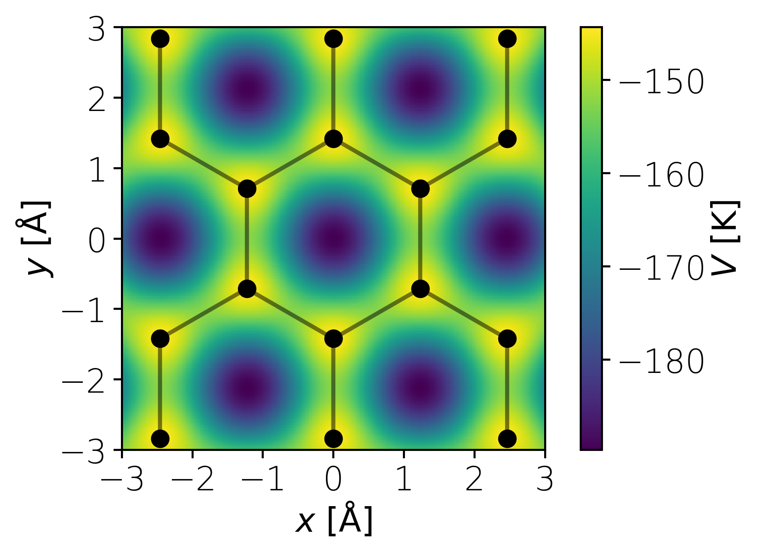
The 2D potential interaction on the Cartesian plan is generated using the get_V2D() function and takes the generated 2D lookup table as a parameter. Plots of the 2D potential can be generated using plot_V2D() with the option to include the graphene lattice.
# Here we generate 2D potential data on the Cartesian plane by using a generated lookup table
box_dims = gt.np.array([-3.0,3.0,-3.0,3.0])
resolution = 201
fn = "helium-graphene-2D-unit-cell_V_strain_0.00000_z_2.52369_res_101.npz"
big_V, big_xy_x, big_xy_y, extent = gt.get_V2D(fn,box_dims,resolution=resolution)
V2D_data = (big_V, big_xy_x, big_xy_y, extent)

# and plot the data we just generated
dpi = 300
plot_filename="V2D.png" # save plot as this name
mplstylefile = 'default'
fig_ax = None
graphene_lattice = True # include the graphene lattice
try:
    fig, ax, V2D_data = gt.plot_V2D(fn,box_dims,V2D_data=V2D_data,plot_filename=plot_filename,mplstylefile=mplstylefile,resolution=resolution,dpi=dpi)
except:
    fig, ax, V2D_data = gt.plot_V2D(fn,box_dims,plot_filename=plot_filename,mplstylefile=mplstylefile,resolution=resolution,dpi=dpi)
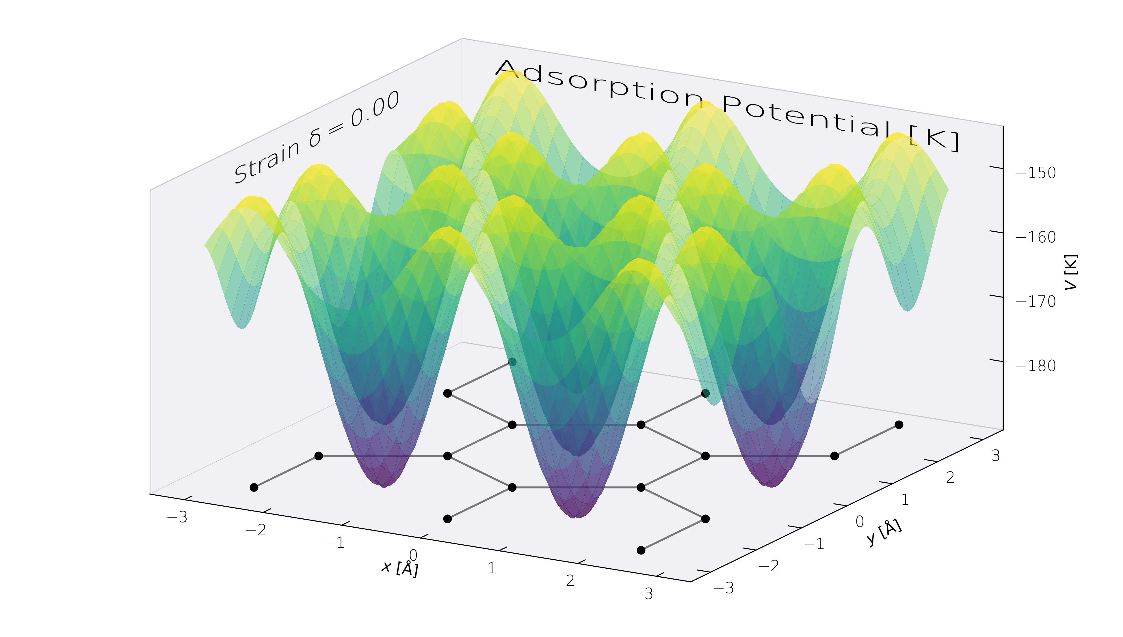
3D potential plot (still a 2D slice)
Similar to the 2D methods a 3D plot of the 2D potential slice can be generated using plot_V3D().
# Here we generate 2D potential data on the Cartesian plane by using a generated lookup table
box_dims = gt.np.array([-3.0,3.0,-3.0,3.0])
resolution = 201
fn = "helium-graphene-2D-unit-cell_V_strain_0.00000_z_2.52369_res_101.npz"
big_V, big_xy_x, big_xy_y, extent = gt.get_V2D(fn,box_dims,resolution=resolution)
V2D_data = (big_V, big_xy_x, big_xy_y, extent)

# and plot the data we just generated
figsize = (16,9) # widescreen!
dpi = 240 # dpi corresponds to 4K image
plot_filename="V3D.png"
mplstylefile = 'default'
fig_ax = None
graphene_lattice = True
surf_kwargs={"alpha":0.5,"cmap":"viridis"}
try:
    fig, ax, V2D_data = gt.plot_V3D(fn,box_dims,plot_filename=plot_filename,V2D_data=V2D_data,mplstylefile=mplstylefile,resolution=resolution,dpi=dpi,figsize=figsize,surf_kwargs=surf_kwargs)
except:
    fig, ax, V2D_data = gt.plot_V3D(fn,box_dims,plot_filename=plot_filename,mplstylefile=mplstylefile,resolution=resolution,dpi=dpi,figsize=figsize,surf_kwargs=surf_kwargs)
Additional usage
See function documentation to discover additional usage.
2 maintainers


Metadata
2 maintainers
Release files for graphenetools-py 0.10.0
For a detailed explanation of source distributions (sdists) and built distributions (wheels), please see the package formats documentation.
Source distribution (sdist)
| File | Size | Uploaded | |
|---|---|---|---|
| graphenetools-py-0.10.0.tar.gz | 18.7 kB | Details |
Built distribution (wheel)
| File | Interpreter | ABI | Platform | Reset |
|---|---|---|---|---|
| graphenetools_py-0.10.0-py3-none-any.whl | Python 3 | none | any | Details |
Total release size: 37.9 kB
Release files / graphenetools-py-0.10.0.tar.gz
| Download URL | graphenetools-py-0.10.0.tar.gz |
|---|---|
| Size | 18.7 kB |
| Tags | Source |
|
SHA-256 checksum How to use checksums |
85fdec58fe7b70d1b7ce178bde1904419a5558ed2f84e3bc506c98e13f3b314f
|
|
BLAKE2b-256 checksum How to use checksums |
7bde3b0d7a491121958f8c5d5b51389ea8d0ee53dc42fa93bf3a699005b6ff43
|
| Upload date | |
|
Uploaded using Trusted Publishing? What is trusted publishing? |
No |
| Uploaded via |
twine/3.4.2 importlib_metadata/4.0.1 pkginfo/1.7.1 requests/2.25.1 requests-toolbelt/0.9.1 tqdm/4.59.0 CPython/3.9.1
|
Release files / graphenetools_py-0.10.0-py3-none-any.whl
| Download URL | graphenetools_py-0.10.0-py3-none-any.whl |
|---|---|
| Size | 19.2 kB |
| Tags | Python 3 |
|
SHA-256 checksum How to use checksums |
94168f4869d377d256ac02b16df7eb1625cc4fb246459fee43f742b85885a7a6
|
|
BLAKE2b-256 checksum How to use checksums |
8979c97b2071fdf082d65aaf89562b48ffb67add1053573e704874f81fcb1f58
|
| Upload date | |
|
Uploaded using Trusted Publishing? What is trusted publishing? |
No |
| Uploaded via |
twine/3.4.2 importlib_metadata/4.0.1 pkginfo/1.7.1 requests/2.25.1 requests-toolbelt/0.9.1 tqdm/4.59.0 CPython/3.9.1
|














