
❒ Gridpoints — Multi dimensional sort for point clouds
Gridpoints maps raw indexes of unstructured point clouds to structured grids multi-index through a bijective transformation:
One point, one cell,
n <-> [i,j,…](n).
It replaces and enhances the squarenet project with a more robust points sorting algorithm. The goal is to build a spatialy coherent multi index to later store and query the point cloud efficiently, based on adaptative axes (lines, columns, and more in 3D+) as showed on following exemple :
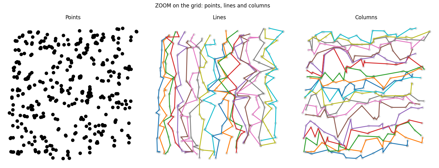
What it does: Take raw point cloud P(N, D) and find a grid shape and an index permutation order such that Pgrid(I, J, …, D) = P[order].reshape(*gridshape, D) is sorted along every axis of the grid. E.g. in 3D, for Pgrid = (x, y, z):
x[i+1, j, k] >= x[i, j, k]
y[i, j+1, k] >= y[i, j, k]
z[i, j, k+1] >= z[i, j, k]
→ On the Pgrid view of P, neighbor queries become a simple stencil look-up
neighborhood(Pgrid[i, j, k]) = {Pgrid[i±di, j±dj, k±dk] | (di, dj, dk) ≤ R},
where R is a radius cutoff to determine, allowing local operations in linear time.
→ Geometric operations (convolution, clustering, interpolation …) can then be applied in linear time directly on the Pgrid view instead of relying on complex graph or point-cloud methods
P can be a NumPy, PyTorch or CuPy array of any dimension (N, D). To allow natural padding when the grid has more cells than they are points in the cloud, NaNs and Infs are supported in a consistent manner:
- nans → random position
- (+-) infs → border of the grid
This allow to gridsort prime or variable number of points, as long as one is ready to deal with void/special grid cells.
Expected runtime for sorting 1 million points: CPU: < 10s (numpy), GPU: < 500 ms (torch cuda)
When not to use gridpoints ?
- high dimension: the package is implemented to support arbitrary dimension, but sweetspot is really 2D/3D. dimensions 4-6 might still be reasonable depending on the task, but anything above 8D is generally too high dimensional for gridpoints.
- weird geometries. Supported datasets goes beyond smooth convex distributions: map of Indonesia, a sponge, a donuts, an elephant, an eggshell (by specifying a suitable gridshape e.g. (128,128,2) to
gridpoints.sort()). You can see various exemples in the plot folder But with some limits. Bad fits: a spider web, a wind turbine, same eggshell with a naive 3d sort (gridshape = (32,32,32)) ... the issue is not that gridpoints cannot sort these distributions, but that it will produce a poor representation of the geometry. - small point clouds: beyond a few hundred points, local operations in linear time is not worth the overhead, because naive quadratic implementations will probably be simultaneously simpler and faster.
Installation
pip install gridpoints          # core only
pip install gridpoints[demo]    # for the demonstration notebook.
Full Demo: notebook.ipynb
Quickstart
import gridpoints as grid
import numpy as np

# Raw point cloud (numpy, pytorch or cupy)
A = np.random.rand(1_000_000, 3)

# Sorted view: place the points inside the grid
order = grid.argsort(A, gridshape=(100, 100, 100))
Bflat = A[order] #flat but sorted with a grid layout (C-order)
Bgrid = Bflat.reshape(100, 100, 100, 3) #reshaped as a grid

# Rest of your pipeline, working with grids
Cgrid = apply_something(Bgrid) #(100, 100, 100, *)

# Back to the original points indexing
Cflat = Cgrid.reshape(1_000_000, *)
orderinv = grid.invert_permutation(order)
C = Cflat[orderinv]   # matches the initial points order
Note on rectangular gridshapes
The eggshell example illustrates the importance of selecting a suitable grid-shape decomposition. This can itself be challenging when the point cloud is assumed to follow a complex topological pattern, such as a thin surface rather than a full volumetric domain. While the precise decomposition is not particularly important (e.g. (18,20,16) vs. (16,15,24) will generally make little difference), the orders of magnitude of the different dimensions do matter and should be tuned to the dataset: (18,20,16) and (36,40,4) can lead to substantially different results. As mentioned, nan/inf padding can help accomodate integer-factorization constraints
Another possibility for smoothing out topology-specific effects is to perform the sort after randomly projecting the dataset onto a lower-dimensional subspace. Random projections are known to approximately preserve pairwise distances, as formalized by the Johnson–Lindenstrauss lemma.
Note on the cutoff radius R
There is no strict theoretical guarantee about what the cutof radius R should be for a given task. E.g the relative grid position between a point and its nearest neighbors can't be garanted to be in the exact adjacent grid cells. What is guaranteed from the sorted ordering is only grid monotonicity: x coordinates increase along rows, y coordinates along columns, and so on.
As an example, empirical results in 2-D show that R = 5 is enough for ~99 % of the nearest neighbors; some outlier neighbors will sit further apart for complex geometries with pronounced peaks, holes or any non-smoothness. When a stricter neighborhood is required, or in high dimensional setting, the solution might be to build an assembly of grid experts, each working on a rotated / projected view of the points, as discussed in this topic. An other possibility would be to tile the grid: each tile is enhanced with location metadata (e.g. a bounding box), allowing for pruning pairs of tiles with a distance certified to be far enough for a given criterion.
Note on efficient stencil operations
The typical use-case of Gridpoints is to allow fast local operations on arbitrary point clouds using stencil kernels:
output(i, j, k) = f( Pgrid[i±di, j±dj, k±dk] | di, dj, dk in local window )
To go beyond standard (slow) python loops, this kind of kernel computation can be accelerated with native grid convolution operations of standard libraries whenever possible, or with pystencils or taichi compilers for complex/non linear grid kernels. On GPU, tiling the grid and leveraging a custom triton kernel might be particularly efficient.
1 maintainer

Metadata
1 maintainer
Release files for gridpoints 1.0.7
For a detailed explanation of source distributions (sdists) and built distributions (wheels), please see the package formats documentation.
Source distribution (sdist)
| File | Size | Uploaded | |
|---|---|---|---|
| gridpoints-1.0.7.tar.gz | 17.6 kB | Details |
Built distribution (wheel)
| File | Interpreter | ABI | Platform | Reset |
|---|---|---|---|---|
| gridpoints-1.0.7-py3-none-any.whl | Python 3 | none | any | Details |
Total release size: 33.5 kB
Release files / gridpoints-1.0.7.tar.gz
| Download URL | gridpoints-1.0.7.tar.gz |
|---|---|
| Size | 17.6 kB |
| Tags | Source |
|
SHA-256 checksum How to use checksums |
e959120567b93569811ef3455aab72797251ce74ab19e46c90e5ec3d3cecae3e
|
|
BLAKE2b-256 checksum How to use checksums |
4aa13ba9f8f4c6f7e3f61588402da31eaab142bdd04b5518b396de8b90abc381
|
| Upload date | |
|
Uploaded using Trusted Publishing? What is trusted publishing? |
No |
| Uploaded via |
twine/7.0.0 CPython/3.14.4
|
Release files / gridpoints-1.0.7-py3-none-any.whl
| Download URL | gridpoints-1.0.7-py3-none-any.whl |
|---|---|
| Size | 15.9 kB |
| Tags | Python 3 |
|
SHA-256 checksum How to use checksums |
104fd9704e810780082db8a7f9d56fddb52eaf45030e52cc5652c345eb1401d9
|
|
BLAKE2b-256 checksum How to use checksums |
dc6a0413c92fb540f011576b60fd3d8c52bf66ac19d2a8ec5570c2101d21a61e
|
| Upload date | |
|
Uploaded using Trusted Publishing? What is trusted publishing? |
No |
| Uploaded via |
twine/7.0.0 CPython/3.14.4
|














